<?xml version="1.0" encoding="utf-8"?><feed xmlns="http://www.w3.org/2005/Atom" ><generator uri="https://jekyllrb.com/" version="4.4.1">Jekyll</generator><link href="https://francesco.ballerin.it/feed.xml" rel="self" type="application/atom+xml" /><link href="https://francesco.ballerin.it/" rel="alternate" type="text/html" /><updated>2026-07-29T11:03:05+00:00</updated><id>https://francesco.ballerin.it/feed.xml</id><title type="html">Francesco Ballerin</title><subtitle>Personal website of Francesco Ballerin</subtitle><entry><title type="html">Simulating chaos: the Kuramoto–Sivashinsky equation</title><link href="https://francesco.ballerin.it/2026/06/19/kuramoto-sivashinsky-simulator.html" rel="alternate" type="text/html" title="Simulating chaos: the Kuramoto–Sivashinsky equation" /><published>2026-06-19T00:00:00+00:00</published><updated>2026-06-19T00:00:00+00:00</updated><id>https://francesco.ballerin.it/2026/06/19/kuramoto-sivashinsky-simulator</id><content type="html" xml:base="https://francesco.ballerin.it/2026/06/19/kuramoto-sivashinsky-simulator.html"><![CDATA[<h2 id="motivation">Motivation</h2>

<p>In the spring of 2026 I started to work on data-driven discovery of PDEs as part of my PhD project, with a focus on equivariant methods for PDE discovery on flat planes, spheres, and hyperplanes. Instead of deriving equations from physical principles the idea is to start from data and try to deduce the governing equations. This is fairly well studied, but the question of how to handle the same problem when symmetries are known (or suspected) or when the domain has non-zero curvature was still unexplored.</p>

<p>Erlend (my doctoral advisor) and I had already worked on the foundations of this problem from the theoretical side, by studying a complete classification of equivariant polynomial differential operators <sup id="fnref:1"><a href="#fn:1" class="footnote" rel="footnote" role="doc-noteref">1</a></sup>, and we wanted to now apply our results to a practical problem. I started by designing a research plan which involved picking some famous PDEs to test, implementing a numerical integrator to simulate them, and applying our methods against known benchmarks. Doing a literature review, one of the PDEs I encountered was the Kuramoto–Sivashinsky (KS) equation <sup id="fnref:2"><a href="#fn:2" class="footnote" rel="footnote" role="doc-noteref">2</a></sup>,<sup id="fnref:3"><a href="#fn:3" class="footnote" rel="footnote" role="doc-noteref">3</a></sup>, and I was immediately fascinated by it!</p>

<p>The KS equation is one of the simplest partial differential equations that exhibits several regimes among which some are <strong>spatiotemporal chaos</strong>. It is a canonical testbed for studying chaos in extended systems, and it appears in surprisingly many physical contexts.</p>

<p>What struck me most was the dramatic change in behaviour (the different patterns) as a single parameter (the domain size \(L\)) is varied. For small domains the equation is boring as everything decays to zero, but for slightly larger domains, steady cellular patterns emerge (hexagons, rolls, or oscillating cells). Push \(L\) further, and the cells break apart into fully developed spatiotemporal chaos. Three qualitatively different regimes from one parameter. I wanted to <em>see</em> them, and I wanted to <em>play</em> with them. I then needed to write my own simulator to do that, and I decided to build it as a browser-based interactive tool for everyone to enjoy.</p>

<p>This post walks through the equation, the three regimes, and briefly how the simulator works under the hood. You can play with it yourself <a href="https://francesco.ballerin.it/ks_equation">here</a>.</p>

<hr />

<h2 id="the-equation-in-1d">The equation in 1D</h2>

<p>Before diving into two dimensions, it's worth looking at the one-dimensional version. In 1D the KS equation is usually written as</p>

\[\partial_t u + \partial_x^2 u + \partial_x^4 u + \frac{1}{2}(\partial_x u)^2 = 0,\qquad x \in [0, L], \quad \text{periodic}.\]

<p>To understand what each term does, we switch to Fourier space (where \(\partial_x \to i k\), turning derivatives into multiplication). Expanding \(u(x,t) = \sum_k \hat{u}_k(t) e^{i k x}\) with \(k = 2\pi j / L\) for \(j \in \mathbb{Z}\), the equation becomes</p>

\[\partial_t \hat{u}_k = (k^2 - k^4)\hat{u}_k + \hat{N}(u)_k,\]

<p>where the linear part breaks down as follows:</p>

<table>
  <thead>
    <tr>
      <th>Physical space</th>
      <th>Fourier space</th>
      <th>Effect</th>
    </tr>
  </thead>
  <tbody>
    <tr>
      <td>\(-\partial_x^2 u\)</td>
      <td>\(k^2 \hat{u}_k\)</td>
      <td>anti-diffusion (amplifies)</td>
    </tr>
    <tr>
      <td>\(-\partial_x^4 u\)</td>
      <td>\(-k^4 \hat{u}_k\)</td>
      <td>hyperdiffusion (damps)</td>
    </tr>
  </tbody>
</table>

<p>The two linear terms compete: \(k^2\) wants to grow the mode, \(-k^4\) wants to kill it. Modes with \(\vert k\vert &lt; 1\) grow (anti-diffusion wins), modes with \(\vert k\vert &gt; 1\) decay (hyperdiffusion wins). The nonlinear term \(\hat{N}(u)_k = \mathcal{F}[-\tfrac{1}{2}(\partial_x u)^2]\) couples different \(k\) together, transferring energy between scales.</p>

<p>The classic way to visualize the 1D KS equation is through a <strong>spacetime plot</strong>: a horizontal slice of the solution stacked vertically over time.</p>

<div class="w3-row">
    <figure class="w3-col w3-center l12 m12 s12 blogpost-figure">
        <img src="https://upload.wikimedia.org/wikipedia/commons/7/71/Kuramoto%E2%80%93Sivashinsky_spatiotemporal_evolution.png" alt="Spatiotemporal evolution of the 1D Kuramoto–Sivashinsky equation. The horizontal axis is space, the vertical axis is time running upward. Image by Eviatar Bach, CC0, via &lt;a href='https://commons.wikimedia.org/wiki/File:Kuramoto%E2%80%93Sivashinsky_spatiotemporal_evolution.png'&gt;Wikimedia Commons&lt;/a&gt;." class="blogpost-image" />
        <figcaption class="caption blogpost-caption">Spatiotemporal evolution of the 1D Kuramoto–Sivashinsky equation. The horizontal axis is space, the vertical axis is time running upward. Image by Eviatar Bach, CC0, via <a href="https://commons.wikimedia.org/wiki/File:Kuramoto%E2%80%93Sivashinsky_spatiotemporal_evolution.png">Wikimedia Commons</a>.</figcaption>
    </figure>
</div>

<hr />

<h2 id="the-equation-in-2d">The equation in 2D</h2>

<p>In two spatial dimensions the KS equation takes the form</p>

\[\partial_t u = -\nabla^2 u - \nu \nabla^4 u - \frac{1}{2}\vert\nabla u\vert^2,\qquad(x,y) \in [0, L]^2, \quad \text{periodic}.\]

<p>The parameter \(\nu\) controls the strength of the hyperdiffusion (in the 1D version above, \(\nu\) was implicitly set to 1).</p>

<p>To analyze the equation, we expand the solution in a 2D Fourier series. Because the domain is periodic, we can write</p>

\[u(x,y,t) = \sum_{\mathbf{k}} \hat{u}_{\mathbf{k}}(t)\, e^{i(k_x x + k_y y)},\]

<p>where the index of the Fourier coefficients \(\mathbf{k} = (k_x, k_y)\) is called <strong>wavevector</strong>, which label each Fourier mode. The magnitude \(k = \vert\mathbf{k}\vert = \sqrt{k_x^2 + k_y^2}\) is called the <strong>wavenumber</strong>. A mode with large \(k\) varies rapidly in space (small ripples), while a mode with small \(k\) varies slowly (broad swells). The coefficient \(\hat{u}_{\mathbf{k}}(t)\) is a complex number encoding the amplitude and phase of the mode with wavevector \(\mathbf{k}\) at time \(t\).</p>

<p>Working in Fourier space turns derivatives into multiplication, and just as \(\partial_x\) turns into \(i k_x\) in 1D, in 2D the gradient becomes \(i\mathbf{k} = (i k_x, i k_y)\), and the Laplacian becomes \(-\vert\mathbf{k}\vert^2 = -(k_x^2 + k_y^2)\). Applying this to the KS equation, we split it into a linear part \((-\Delta u - \nu\Delta^2 u)\) and a nonlinear part \((-\tfrac{1}{2}\vert\nabla u\vert^2)\), and transform each:</p>

<ul>
  <li>The linear part becomes \(\bigl(\vert\mathbf{k}\vert^2 - \nu\vert\mathbf{k}\vert^4\bigr)\,\hat{u}_{\mathbf{k}}\). Crucially, this is <strong>diagonal</strong>: each Fourier mode \(\hat{u}_{\mathbf{k}}\) is multiplied only by a scalar that depends on \(\mathbf{k}\) alone. There is no mixing between different \(\mathbf{k}\) — mode \(\mathbf{k}\) doesn't talk to mode \(\mathbf{k}'\) through the linear terms.</li>
  <li>The nonlinear part, which we write as \(\hat{N}(u)_{\mathbf{k}} = \mathcal{F}\bigl[-\tfrac{1}{2}\vert\nabla u\vert^2\bigr]\), is <em>not</em> diagonal: it couples different Fourier modes through convolution. This coupling is what transfers energy between scales and ultimately generates chaos.</li>
</ul>

<p>So in Fourier space the PDE becomes a system of ordinary differential equations, one for each \(\mathbf{k}\):</p>

\[\partial_t \hat{u}_{\mathbf{k}} = \bigl(\vert\mathbf{k}\vert^2 - \nu\vert\mathbf{k}\vert^4\bigr)\,\hat{u}_{\mathbf{k}} \;+\; \hat{N}(u)_{\mathbf{k}}.\]

<p>The linear coefficient depends only on \(k = \vert\mathbf{k}\vert\), so the linear part is diagonal — each mode evolves independently. Because it is diagonal, the linear part can be solved exactly: over a time step \(h\), each mode simply multiplies by</p>

\[\hat{u}_{\mathbf{k}}(t + h) = e^{(k^2 - \nu k^4)h} \,\hat{u}_{\mathbf{k}}(t),
\qquad\text{where } k = \vert\mathbf{k}\vert.\]

<p>Just as in 1D, the growth rate \(k^2 - \nu k^4\) pits anti-diffusion (\(k^2\), wants to grow) against hyperdiffusion (\(-\nu k^4\), wants to decay). The two balance at the <strong>critical wavenumber</strong></p>

\[k_{\text{crit}} = \frac{1}{\sqrt{\nu}}.\]

<p>Modes with \(k &lt; k_{\text{crit}}\) grow; modes with \(k &gt; k_{\text{crit}}\) decay.</p>

<p>What does this have to do with the domain size? On a periodic domain of length \(L\), the smallest nonzero wavenumber is \(k_{\min} = 2\pi/L\) and you can't fit a wave longer than the box in the box itself. If even this longest wave decays (\(k_{\min} &gt; k_{\text{crit}}\)), the solution dies out. The threshold \(k_{\min} = k_{\text{crit}}\) gives the critical domain size</p>

\[L^\ast = 2\pi\sqrt{\nu}.\]

<hr />

<h2 id="three-regimes-one-equation">Three regimes, one equation</h2>

<p>The ratio \(L / L^\ast\) is the single parameter that determines the qualitative behaviour of the system. Here's what happens as you increase it.</p>

<h3 id="stable-l--last">Stable (\(L &lt; L^\ast\))</h3>

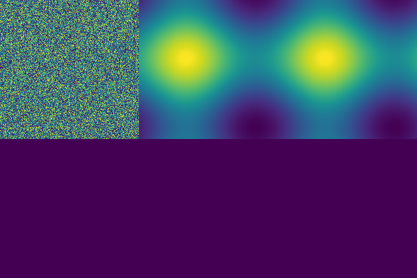
<p>When the domain is smaller than the critical length, no Fourier mode fits within the unstable band. Every mode decays exponentially, and any initial condition eventually flattens to \(u \equiv 0\). Not terribly exciting, but a good sanity check for the simulator.</p>

<div class="w3-row">
    <figure class="w3-col w3-center l12 m12 s12 blogpost-figure">
        <img src="/assets/images/blogposts/ks-equation/stable.gif" alt="Stable regime: L = 2, ν = 1. The initial random noise decays to a uniform field." class="blogpost-image" />
        <figcaption class="caption blogpost-caption">Stable regime: L = 2, ν = 1. The initial random noise decays to a uniform field.</figcaption>
    </figure>
</div>

<h3 id="cellular-last--l-lesssim-3last">Cellular (\(L^\ast &lt; L \lesssim 3L^\ast\))</h3>

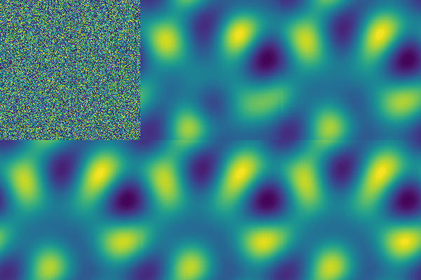
<p>A small set of modes — those whose wavevectors fit inside the unstable annulus \(0 &lt; \vert\mathbf{k}\vert &lt; 1/\sqrt{\nu}\) — begin to grow. Nonlinear saturation locks them into steady or periodically oscillating patterns: rolls, hexagons, or mixed states depending on the initial condition and the precise value of \(L\).</p>

<div class="w3-row">
    <figure class="w3-col w3-center l12 m12 s12 blogpost-figure">
        <img src="/assets/images/blogposts/ks-equation/cellular.gif" alt="Cellular regime: L = 10, ν = 1. A hexagonal pattern emerges from random noise and stabilises into a steady cellular structure." class="blogpost-image" />
        <figcaption class="caption blogpost-caption">Cellular regime: L = 10, ν = 1. A hexagonal pattern emerges from random noise and stabilises into a steady cellular structure.</figcaption>
    </figure>
</div>

<h3 id="chaotic-l-gg-last">Chaotic (\(L \gg L^\ast\))</h3>

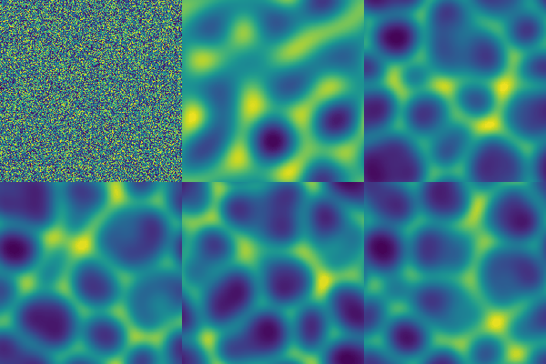
<p>When the domain supports many unstable modes, the nonlinear term transfers energy between them continuously and the patterns never settle. They twist, merge, split, and reform in an endless dance which is <strong>spatiotemporal chaos</strong>. The field at any given point fluctuates unpredictably and produces a result that is visually mesmerising.</p>

<div class="w3-row">
    <figure class="w3-col w3-center l12 m12 s12 blogpost-figure">
        <img src="/assets/images/blogposts/ks-equation/chaotic.gif" alt="Chaotic regime: L = 30, ν = 1. The field never settles into a steady pattern; structures continuously form, interact, and dissolve." class="blogpost-image" />
        <figcaption class="caption blogpost-caption">Chaotic regime: L = 30, ν = 1. The field never settles into a steady pattern; structures continuously form, interact, and dissolve.</figcaption>
    </figure>
</div>

<hr />

<h2 id="how-the-simulator-works">How the simulator works</h2>

<p>The simulator runs entirely in the browser with the use of a JavaScript snippet. The numerical engine is implemented from scratch following standard methods from the literature, with some tweaks to balance accuracy and performance.</p>

<p>Halfway through the project I came across <a href="https://observablehq.com/@rreusser/kuramoto-sivashinsky-equation-in-2d">Ricky Reusser's beautiful WebGL notebook</a> which implements a similar simulator, which I recommend checking out. Especially his WebGPU implementation which is incredibly fast.</p>

<p>Here's a high-level overview of the key components of the simulator I built. I am not an expert in numerical PDEs, so a lot of the design choices were made through trial and error and relying on papers I scavenged from the internet. If you have suggestions for improvements, please let me know!</p>

<h3 id="spectral-discretization">Spectral discretization</h3>

<p>The domain \([0, L]^2\) is discretised into an \(M \times M\) grid. Since the boundary conditions are periodic, the natural basis is the Fourier basis. The solution is represented by its Fourier coefficients \(\hat{u}_{\mathbf{k}}\) on a grid of wavenumbers</p>

\[\mathbf{k} \in \frac{2\pi}{L}\big\{(j_x, j_y) \;\big\vert\; j_x, j_y = 0, \pm 1, \dots, \pm M/2\big\}.\]

<p>Spatial derivatives are computed in Fourier space (multiplication by \(i k_x\) or \(i k_y\)), then transformed back to physical space when needed. The 2D FFT is the workhorse — specifically a hand-written radix-2 Cooley–Tukey implementation. It's not as fast as FFTW, but it runs in a Web Worker so the UI stays responsive.</p>

<h3 id="the-nonlinear-term">The nonlinear term</h3>

<p>The nonlinear term \(\hat{N}(u) = \mathcal{F}[-\frac{1}{2}\vert\nabla u\vert^2]\) is computed <em>pseudo-spectrally</em>:</p>

<ol>
  <li>Compute the physical-space gradient \(\nabla u = \mathcal{F}^{-1}[i\mathbf{k}\,\hat{u}]\)</li>
  <li>Form \(-\frac{1}{2}\vert\nabla u\vert^2\) pointwise in physical space</li>
  <li>Transform back: \(\hat{N} = \mathcal{F}[-\frac{1}{2}\vert\nabla u\vert^2]\)</li>
</ol>

<p>Apparently, there can be an issue of aliasing, which can be addressed by the <strong>2/3 de-aliasing rule</strong>: after each step, zero out all Fourier modes with \(\vert j_x\vert &gt; M/3\) or \(\vert j_y\vert &gt; M/3\). This removes the aliasing error at the cost of effectively running on a coarser grid (and about a 2× slowdown). In practice, I don't really see much difference.</p>

<h3 id="exponential-time-differencing-etd">Exponential Time Differencing (ETD)</h3>

<p>The hyperdiffusion term \(-\nu\nabla^4 u\) is extremely <strong>stiff</strong>. A stiff term is one that involves drastically different time scales within the same problem and here, the high-wavenumber modes decay orders of magnitude faster than the low-wavenumber ones. Any explicit time-stepping method must take steps small enough to resolve the <em>fastest</em> scale, even if we only care about the slow ones.</p>

<p>Concretely, let's see what happens if we try to use forward Euler. For the highest resolved wavenumber \(\vert\mathbf{k}\vert_{\max} \approx \pi M/L\) the hyperdiffusion term \(-\nu\vert\mathbf{k}\vert^4 \hat{u}\) contributes \(-\nu(\pi M/L)^4\). An explicit method would require \(\Delta t \sim 1/\vert\mathbf{k}\vert_{\max}^4 \sim L^4/(\nu M^4)\) for stability. On a modest \(64 \times 64\) grid, that's around \(10^{-6}\). We would need a million steps to simulate one time unit. A bit pricey.</p>

<p>The solution: treat the <em>linear</em> part exactly. Write the PDE in Fourier space as</p>

\[\partial_t \hat{u} = \hat{L} \hat{u} + \hat{N}(u),\]

<p>where \(\hat{L} = \text{diag}(\vert\mathbf{k}\vert^2 - \nu\vert\mathbf{k}\vert^4)\). The exact solution over a time step \(h\) satisfies</p>

\[\hat{u}(t+h) = e^{\hat{L}h}\,\hat{u}(t) + \int_0^h e^{\hat{L}(h-\tau)}\,\hat{N}(u(t+\tau))\,d\tau.\]

<p>The first term handles the linear part <strong>exactly</strong> with no stability restriction from the \(\vert\mathbf{k}\vert^4\) term. The integral involving the nonlinearity is approximated by a Runge–Kutta scheme, giving a family of <strong>Exponential Time Differencing</strong> methods. The specific one used here is <strong>ETDRK4</strong> <sup id="fnref:4"><a href="#fn:4" class="footnote" rel="footnote" role="doc-noteref">4</a></sup>, a fourth-order scheme. Its coefficients involve the \(\varphi\)-functions, which arise naturally from the integral in the exact solution formula:</p>

\[\begin{aligned}
\varphi_0(z) &amp;= e^z, &amp;
\varphi_1(z) &amp;= \frac{e^z - 1}{z}, \\[4pt]
\varphi_2(z) &amp;= \frac{e^z - 1 - z}{z^2}, &amp;
\varphi_3(z) &amp;= \frac{e^z - 1 - z - z^2/2}{z^3}.
\end{aligned}\]

<p>The ETDRK4 step reads:</p>

\[\begin{aligned}
a &amp;= \varphi_0(\tfrac{h}{2}\hat{L})\,u_n + \tfrac{h}{2}\varphi_1(\tfrac{h}{2}\hat{L})\,N(u_n), \\
b &amp;= \varphi_0(\tfrac{h}{2}\hat{L})\,u_n + \tfrac{h}{2}\varphi_1(\tfrac{h}{2}\hat{L})\,N(a), \\
c &amp;= \varphi_0(\tfrac{h}{2}\hat{L})\,a + \tfrac{h}{2}\varphi_1(\tfrac{h}{2}\hat{L})\,(2N(b) - N(u_n)), \\
\end{aligned}\]

\[u_{n+1} = \varphi_0(h\hat{L}) u_n + h(\varphi_1-3\varphi_2+4\varphi_3)N(u_n) + h(2\varphi_2-4\varphi_3)(N(a)+N(b)) + h(-\varphi_2+4\varphi_3)N(c),\]

<p>where all \(\varphi_{\ell}\) are evaluated at \(h\hat{L}\) in the final line.</p>

<p>Evaluating \(\varphi_1, \varphi_2, \varphi_3\) near \(z = 0\) requires care — the formulas above suffer from catastrophic cancellation. The simulator uses a numerically stable evaluation <sup id="fnref:6"><a href="#fn:6" class="footnote" rel="footnote" role="doc-noteref">5</a></sup>, falling back to the explicit formula for \(\vert z\vert &gt; 5\) where it is safe.</p>

<p>The simulator also offers a simpler <strong>IMEX BDF2</strong> integrator (implicit-explicit Backward Differentiation Formula, second order). It treats the stiff linear terms implicitly and the nonlinearity explicitly, trading some accuracy for better stability on coarse grids. This is what Reusser's notebook uses.</p>

<h3 id="why-does-it-still-blow-up-sometimes">Why does it still blow up sometimes?</h3>

<p>If you push the domain size too large or the hyperviscosity too low, the simulation will eventually blow up and the solver will stop. This is frustrating, especially if you've seen other KS simulators (notably <a href="https://observablehq.com/@rreusser/kuramoto-sivashinsky-equation-in-2d">Ricky Reusser's beautiful WebGL notebook</a>) that seem to run forever without a hiccup. What gives?</p>

<p><strong>Half-precision arithmetic as accidental hyperviscosity.</strong> Reusser's simulation runs on the GPU using WebGL textures, which default to 16-bit floating point (float16). Every multiplication discards information at high wavenumbers. This acts as an unintentional low-pass filter that continuously damps the very modes most prone to instability. Our solver uses Float64Array (double precision) in a Web Worker, preserving energy across all resolved scales, including the ones that can run away.</p>

<p><strong>A different form of the equation.</strong> Reusser follows Kalogirou et al. <sup id="fnref:5"><a href="#fn:5" class="footnote" rel="footnote" role="doc-noteref">6</a></sup>, who shift the solution by a constant drift: \(V = u - ct\). This introduces a term proportional to \(c\,dt\) into the BDF2 update formula that provides additional damping of previous timesteps. Our implementation solves the KS equation directly without this shift.</p>

<p><strong>Energy-leaking post-processing.</strong> After every timestep, Reusser's code runs an extra cycle to remove imaginary leakage from the complex FFT of real data. Each such pass removes a tiny amount of energy. Our code preserves Hermitian symmetry analytically (if \(\hat{u}_{-\mathbf{k}} = \overline{\hat{u}_{\mathbf{k}}}\), the IFFT is real), so no stripping is needed (but we also don't get the free dissipation).</p>

<p>The IMEX BDF2 integrator mentioned above follows the same approach as Reusser's notebook but without the half-float damping or the \(c\)-shift.</p>

<hr />

<h2 id="try-it-yourself">Try it yourself</h2>

<p>The simulator is live at <strong><a href="https://francesco.ballerin.it/ks_equation">francesco.ballerin.it/ks_equation</a></strong>. Here are some parameter combinations to get you started:</p>

<table>
  <thead>
    <tr>
      <th>Regime</th>
      <th>\(L\)</th>
      <th>\(\nu\)</th>
      <th>\(dt\)</th>
    </tr>
  </thead>
  <tbody>
    <tr>
      <td>Stable</td>
      <td>2</td>
      <td>1.0</td>
      <td>0.25</td>
    </tr>
    <tr>
      <td>Cellular</td>
      <td>10</td>
      <td>1.0</td>
      <td>0.25</td>
    </tr>
    <tr>
      <td>Chaotic</td>
      <td>30</td>
      <td>1.0</td>
      <td>0.25</td>
    </tr>
    <tr>
      <td>Extreme (will rapidly blow up)</td>
      <td>30</td>
      <td>0.1</td>
      <td>0.1</td>
    </tr>
  </tbody>
</table>

<hr />

<h2 id="references">References</h2>

<div class="footnotes" role="doc-endnotes">
  <ol>
    <li id="fn:1">
      <p>Ballerin, F. &amp; Grong, E. (2026). <em>Equivariant nonlinear partial differential operators on constant curvature spaces</em>. <a href="https://arxiv.org/abs/2605.16847">arXiv:2605.16847</a>. <a href="#fnref:1" class="reversefootnote" role="doc-backlink">&#8617;</a></p>
    </li>
    <li id="fn:2">
      <p>Kuramoto, Y. (1978). <em>Diffusion-Induced Chaos in Reaction Systems</em>. Prog. Theor. Phys. Suppl. 64, 346–367. <a href="#fnref:2" class="reversefootnote" role="doc-backlink">&#8617;</a></p>
    </li>
    <li id="fn:3">
      <p>Sivashinsky, G. I. (1977). <em>Nonlinear analysis of hydrodynamic instability in laminar flames—I. Derivation of basic equations</em>. Acta Astronaut. 4, 1177–1206. <a href="#fnref:3" class="reversefootnote" role="doc-backlink">&#8617;</a></p>
    </li>
    <li id="fn:4">
      <p>Cox, S. M. &amp; Matthews, P. C. (2002). <em>Exponential time differencing for stiff systems</em>. J. Comput. Phys. 176, 430–455. <a href="#fnref:4" class="reversefootnote" role="doc-backlink">&#8617;</a></p>
    </li>
    <li id="fn:6">
      <p>Kassam, A.-K. &amp; Trefethen, L. N. (2005). <em>Fourth-order time-stepping for stiff PDEs</em>. SIAM J. Sci. Comput. 26, 1214–1233. <a href="#fnref:6" class="reversefootnote" role="doc-backlink">&#8617;</a></p>
    </li>
    <li id="fn:5">
      <p>Kalogirou, A., Keaveny, E. E. &amp; Papageorgiou, D. T. (2015). <em>An in-depth numerical study of the two-dimensional Kuramoto–Sivashinsky equation</em>. Proc. R. Soc. A 471, 20140932. <a href="#fnref:5" class="reversefootnote" role="doc-backlink">&#8617;</a></p>
    </li>
  </ol>
</div>]]></content><author><name></name></author><category term="projects" /><category term="math" /><category term="simulation" /><summary type="html"><![CDATA[I built an in-browser simulator for the Kuramoto–Sivashinsky equation — one of the simplest PDEs that exhibits spatiotemporal chaos. Here's the math behind it, how the simulator works, and what patterns emerge in different regimes.]]></summary><media:thumbnail xmlns:media="http://search.yahoo.com/mrss/" url="https://francesco.ballerin.it/assets/images/blogposts/ks-equation/chaotic.gif" /><media:content medium="image" url="https://francesco.ballerin.it/assets/images/blogposts/ks-equation/chaotic.gif" xmlns:media="http://search.yahoo.com/mrss/" /></entry><entry><title type="html">Baking frozen pizzas from scratch</title><link href="https://francesco.ballerin.it/2025/12/17/baking-frozen-pizza-from-scratch.html" rel="alternate" type="text/html" title="Baking frozen pizzas from scratch" /><published>2025-12-17T00:00:00+00:00</published><updated>2025-12-17T00:00:00+00:00</updated><id>https://francesco.ballerin.it/2025/12/17/baking-frozen-pizza-from-scratch</id><content type="html" xml:base="https://francesco.ballerin.it/2025/12/17/baking-frozen-pizza-from-scratch.html"><![CDATA[<h1 id="motivation">Motivation</h1>

<p>At some point during one of my productive doomscrolling evenings, on YouTube specifically, I came across a video produced in November 2024 by Marcello Ascani featuring a pizzaiolo who moved to San Francisco, and was at the time working for a company producing Napolitan frozen pizzas in the Bay area. The original video can be found <a href="https://www.youtube.com/watch?v=dzIZ0W0sHI8">here</a>.</p>

<p>The business model showcased in the video was baking fresh Napolitan pizzas just outside of the city, freeze them, and then ship them to around 100 Whole Foods locations in the area, where they were sold at around $10 a piece.</p>

<p>Living in Norway, where frozen pizza is one of the most consumed foods (but alas not because of exceptional quality) this video sparked curiosity in the form of "what if I could do it myself, and have a stack of delicious and cheap homemade frozen pizzas at any given time rather than buying the crap at the store?".</p>

<p>Not that I would buy frozen pizzas anyway. I am a true patriot 🇮🇹🤌.</p>

<hr />

<h1 id="background">Background</h1>

<p>Baking is not a trivial process, and it shares a lot more similarities to chemistry than cooking does. And, believe it or not, chemistry was one of my least favorite subjects in highschool. Probably one of the contributing factors pushing me towards mathematics and informatics rather than physics and engineering.</p>

<p>While preparing for this project I did a deep dive into the theory of flour types and baking — which we are soon going to cover — and contacted a couple of industries dealing in flour milling and frozen pizzas production. The summary of this explorative search follows.</p>

<h3 id="types-of-flours-and-yeast">Types of flours and yeast</h3>

<p>Not all flour is the same, and this is obvious when facing the flour shelf of a well-stocked grocery store. Some flours are sold for breadmaking, others for focaccia, some for cakes and shortbreads. The difference lies not only in the grain type and origin, but also in the milling procedure, and they can be quantified and accurately measured. The characteristics of flours can be inferred by metrics such as protein content, W-value, P/L ratio, water absorption, and ash content just to name a few.</p>

<p>Several countries introduced naming conventions with associated requirements, and have strict regulations on how to name them. In Italy, just to name a country, these types can be defined as <em>tipo 00</em>, <em>tipo 0</em>, <em>tipo 1</em>, <em>tipo 2</em>, and <em>integrale</em>. Other countries may follow different naming conventions.</p>

<h4 id="protein-content">Protein content</h4>

<p>This is the value that is easiest to find as a retail consumer. By law it needs to be reported on every package of flour which is sold. It typical ranges between 9g and 14g per 100g of product. This is usually referred to as the <em>strength</em> of the flour, as the protein contained in the flour is usually gluten-forming proteins.</p>

<p>The rule of thumb is to pick an 11-12.5% for Napolitan pizza and 12.5-14% for long fermentations.</p>

<h4 id="w-value">W-value</h4>

<p>The <em>W-value</em> measures the required energy to deform the dough — either resisting to manipulation or resisting to the dough raising — thus making it a good proxy for gluten strength. The alveograph test consists of inflating a disk of dough, making it into a bubble, until it bursts, while measuring the pressure for the first deformation and the total volume of air that is needed to rupture the glutinic mesh.</p>

<p>Typical ranges and common uses are:</p>
<ul>
  <li>&lt; 170 : weak (cookies and shortbreads)</li>
  <li>180 - 270 : medium (direct doughs, short-medium fermentations)</li>
  <li>280 - 350 : strong (long fermentations)</li>
  <li>&gt; 350 : very strong (panettone, biga for multistep doughs, very high hydration doughs)</li>
</ul>

<p>The W-value is measured in a lab test using the <em>Chopin's alveograph test</em>, and it is not a metric that is legally required to be reported. Approximate ranges can be inferred if the flour is sold as a specific type, but specific values are often found only on more premium flours.</p>

<p>For more refined flours, with a minimal content of bran, the W-value correlates well with the protein content. But for other types of flours, for example wholegrain or if <em>durum wheat</em> or other grains are mixed in, the protein content does not correlate as directly with the W-value as measured by the alveograph test. Moreover, the W-value as a proxy for gluten strength loses significance in these cases and should be disregarded.</p>

<h4 id="pl-ratio">P/L ratio</h4>

<p>The <em>P/L ratio</em> measures the ratio between tenacity (P) and extensibility (L) and it is also measured through the alveograph test. The <em>P value</em> is the pressure to first deformation, while the <em>L value</em> is the total volume of air that the dough can handle before bursting — which corresponds to how much it can extend before rupturing.</p>

<h4 id="ash-content">Ash content</h4>

<p>The <em>ash content</em> is not a measure of how much ash there is in flour, but rather a measure of the mineral content. It has gotten this name due to the procedure with whom it is measured: a sample is burned and minerals are then measured in the ash residue that is left behind after combustion has taken place.</p>

<p>As the minerals are mostly contained in the bran of the wheat, the ash content is a good indicator of how much of the bran has made it into the flour — menaing how little refined the flour is.</p>

<p>In Italy the ash content is regulated by law by the name of the type of the flour, which can be <em>tipo 00</em>, <em>tipo 0</em>, <em>tipo 1</em>, <em>tipo 2</em>, and <em>integrale</em>. In other countries other classifications can be in place, or it can happen that no classification at all is used. In these cases it can be harder to determine the ash content of the flour you are buying.</p>

<hr />

<p>I have attempted to put together a table of some of the flours for sale at retail grocery stores in Norway, as well as online at the specialty store "Oluf Lorentzen". Most of the technical specification of the flour is available online on the websites of the respective producers. I have also contacted Regal flour, which is one of the main brands for retail shoppers in Norway, for information regarding their lines of flour. The price was reported as the minimum "bulk price" for orders of a maximum of 5kg, taking advantage of "quantity discounts" such as 3x2 offers but not seasonal or temporary discounts.</p>

<table>
  <thead>
    <tr>
      <th>Flour</th>
      <th>Protein %</th>
      <th>W-value</th>
      <th>P/L</th>
      <th>Price (NOK/kg)</th>
    </tr>
  </thead>
  <tbody>
    <tr>
      <td>Regal Sifted Wheat Flour</td>
      <td>12%</td>
      <td>?</td>
      <td>?</td>
      <td>14.95</td>
    </tr>
    <tr>
      <td>Molini Pizzuti Tipo 00</td>
      <td>10%</td>
      <td>200</td>
      <td>?</td>
      <td>31.27</td>
    </tr>
    <tr>
      <td>Regal Pizzamel</td>
      <td>12%</td>
      <td>?</td>
      <td>?</td>
      <td>26.50</td>
    </tr>
    <tr>
      <td>La Molisana Tipo 00</td>
      <td>11%</td>
      <td>250</td>
      <td>?</td>
      <td>30.80</td>
    </tr>
    <tr>
      <td>Dallari Tipo 00</td>
      <td>10.2%</td>
      <td>240-270</td>
      <td>?</td>
      <td>31.27</td>
    </tr>
    <tr>
      <td>Caputo Pizzeria</td>
      <td>12.5%</td>
      <td>260-280</td>
      <td>0.50-0.60</td>
      <td>41.27</td>
    </tr>
    <tr>
      <td>Regal Tipo 00</td>
      <td>13%</td>
      <td>260-300</td>
      <td>?</td>
      <td>36.50</td>
    </tr>
    <tr>
      <td>Caputo Nuvola</td>
      <td>12.5%</td>
      <td>270-290</td>
      <td>0.50-0.60</td>
      <td>54.60</td>
    </tr>
    <tr>
      <td>Caputo Saccorosso</td>
      <td>13%</td>
      <td>300-320</td>
      <td>0.50-0.60</td>
      <td>51.20</td>
    </tr>
    <tr>
      <td>Caputo Manitoba oro</td>
      <td>14%</td>
      <td>360-380</td>
      <td>0.45-0.55</td>
      <td>43.93</td>
    </tr>
    <tr>
      <td>Caputo gluten-free</td>
      <td>1%</td>
      <td>?</td>
      <td>?</td>
      <td>161.00</td>
    </tr>
  </tbody>
</table>

<h3 id="choice-of-toppings">Choice of toppings</h3>

<p>Toppings need to be able to preserve their quality when frozen. Sauces, cheeses, roasted vegetables, and cooked meats (pepperoni, 'nduja, bacon …) are all excellent choices as toppings as quality is mostly preserved when undergoing the freezing process. Fresh ingredients and cold cuts, such as rucola, cherry tomatoes, and prosciutto crudo, completely lose their profile when undergoing the freezing and reheating process.</p>

<h3 id="freezing--cold-blast-process">Freezing / cold blast process</h3>

<p>From what I gathered from a quick literature review, it appeared that most of the available research covered (raw) doughs and parbaked (partially baked) products. Parbaking is probably the best way to prepare the pizza dough, but it would deprive the pizza of its classic Napolitan-style crust. I wanted a finished product that was possible to prepare in the oven straight from the freezer in approximately 10-12 minutes.</p>

<p>Research on frozen doughs and parbaked products shows that the type and strength of flour make a big difference in how well the pizza base survives freezing and reheating. Stronger flours with higher gluten content, which correspond to higher W-values, tend to retain more gas and structure after thawing, leading to better texture <sup id="fnref:1"><a href="#fn:1" class="footnote" rel="footnote" role="doc-noteref">1</a></sup>. For home use, this means preferring a strong flour.</p>

<p>If the dough is fully baked — as in our case — freezing can still alter water distribution: ice crystals in the crumb can cause slight dryness, while moisture migration may soften the crust <sup id="fnref:2"><a href="#fn:2" class="footnote" rel="footnote" role="doc-noteref">2</a></sup>. Cold blasting is often used in industrial production, as it drops the temperature of the food quickly, freezing it to the core within minutes. Because freezing happens so fast, the liquids form smaller crystals than they normally would in a regular freezer, locking in structure, texture, and aroma. Unfortunately, this is out of reach for most homecooks. Even without a blast chiller, minimizing the time it takes for the dough to freeze — for example by using thin metal trays — helps protecting the texture and flavor.</p>

<p>From my personal experience a regular freezer is good enough to obtain quite decent results. I have opted to wrap the pizzas in a layer of cling film to avoid freeze burns, which would dramatically reduce the quality of the final product. It is important to let the pizzas cool down before freezing, in order to minimize condensation and raising the internal temperature of the freezer. Optionally, after the pizzas have been frozen solid, it is possible to double wrap them in a second layer of cling film to further decrease the risk of freeze burns when stored for longer periods of time.</p>

<hr />

<h1 id="my-first-attempt">My first attempt</h1>

<p>The recipe I have opted to use is the following, which has a yield of 4 pizzas:</p>

<table>
  <thead>
    <tr>
      <th>Ingredient</th>
      <th>Quantity</th>
      <th>Details</th>
    </tr>
  </thead>
  <tbody>
    <tr>
      <td>Flour</td>
      <td>600 g</td>
      <td>Caputo Pizzeria flour</td>
    </tr>
    <tr>
      <td>Water</td>
      <td>360 g</td>
      <td> </td>
    </tr>
    <tr>
      <td>Oil</td>
      <td>20 g</td>
      <td>Extra-virgin olive oil</td>
    </tr>
    <tr>
      <td>Salt</td>
      <td>14 g</td>
      <td> </td>
    </tr>
    <tr>
      <td>Yeast</td>
      <td>1.5 g</td>
      <td>Caputo dry yeast</td>
    </tr>
  </tbody>
</table>

<p>Napolitan pizza dough does not usually contain oil, but oil is rather used as a topping which is added to the pizza just before going into the oven. However, a bit of extra virgin olive oil makes for a softer and richer dough, which I prefer. It also has the added benefit of makin the dough easier to handle.</p>

<p>After using a kitchen mixer, and giving a final folding by hand, I left the dough to rest and start the raising process at room temperature for approximately 4 hours before moving it in the fridge. This slows down the raising process allowing for better timing.</p>

<p>Approximately 4 hours before the pizza is to be baked, I take the dough out of the fridge and divide it into the 4 portions that will be then used to make the pizzas. After folding the dough a second time, and another 3.5h at room temperature, I like to move the portions again in the fridge to reduce the dough temperature, making the dough a bit stiffer and easier to work.</p>

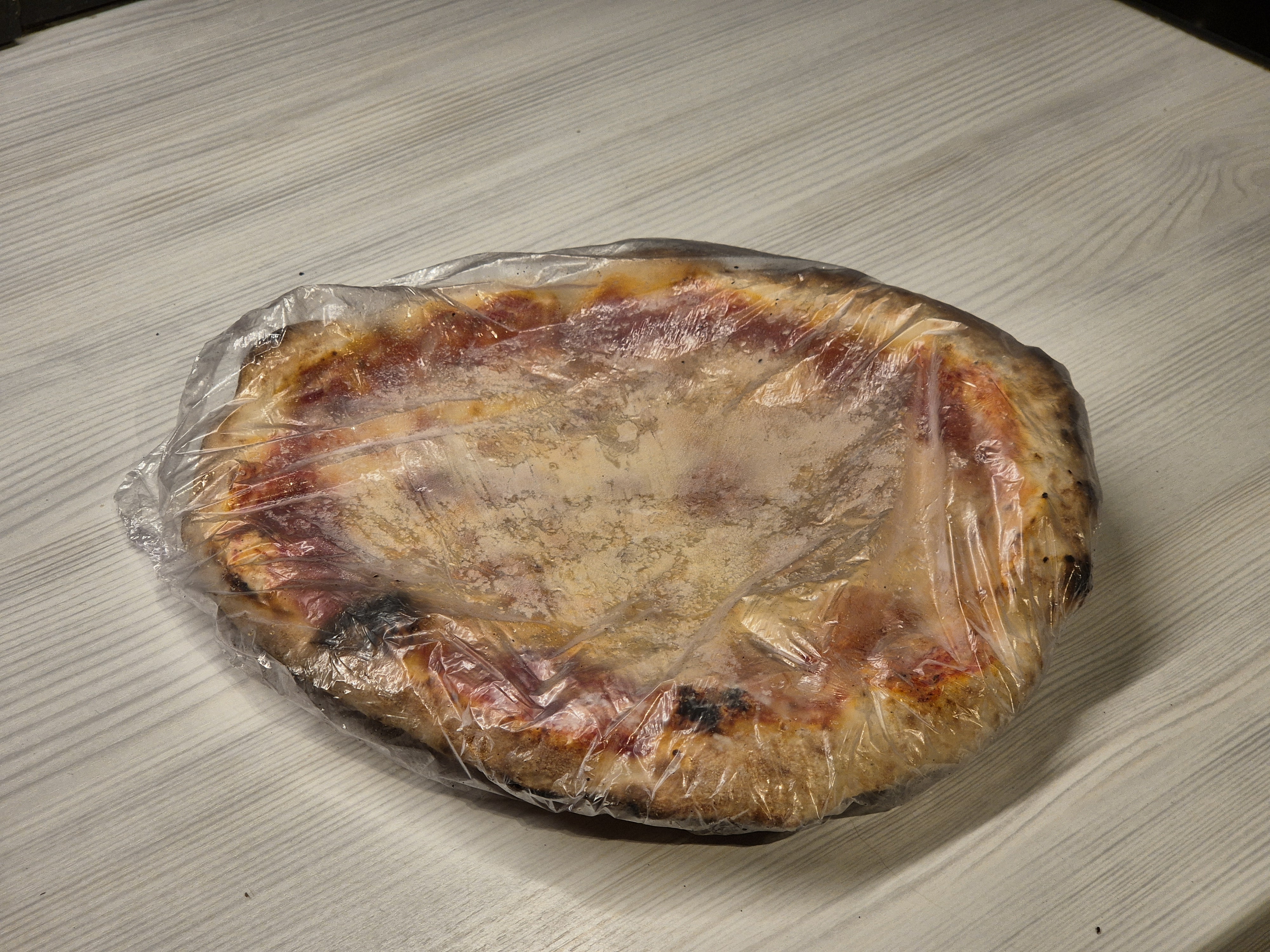
<p>I then baked the pizza in a gas-powered pizza oven (cozze 13") until done, and left it to cool down on the bench before wrapping it in cling foil. As I do not have a chill blaster, I used my freezer to freeze and store the pizza.</p>

<div class="w3-row">
    <figure class="w3-col w3-center l6 m12 s12 blogpost-figure">
        <img src="/assets/images/blogposts/baking-frozen-pizza-from-scratch/first_attempt.jpg" alt="First attempt prior to freezing." class="blogpost-image" />
        <figcaption class="caption blogpost-caption">First attempt prior to freezing.</figcaption>
    </figure>

    <figure class="w3-col w3-center l6 m12 s12 blogpost-figure">
        <img src="/assets/images/blogposts/baking-frozen-pizza-from-scratch/first_attempt_underside.jpg" alt="Underside of the pizza." class="blogpost-image" />
        <figcaption class="caption blogpost-caption">Underside of the pizza.</figcaption>
    </figure>
</div>

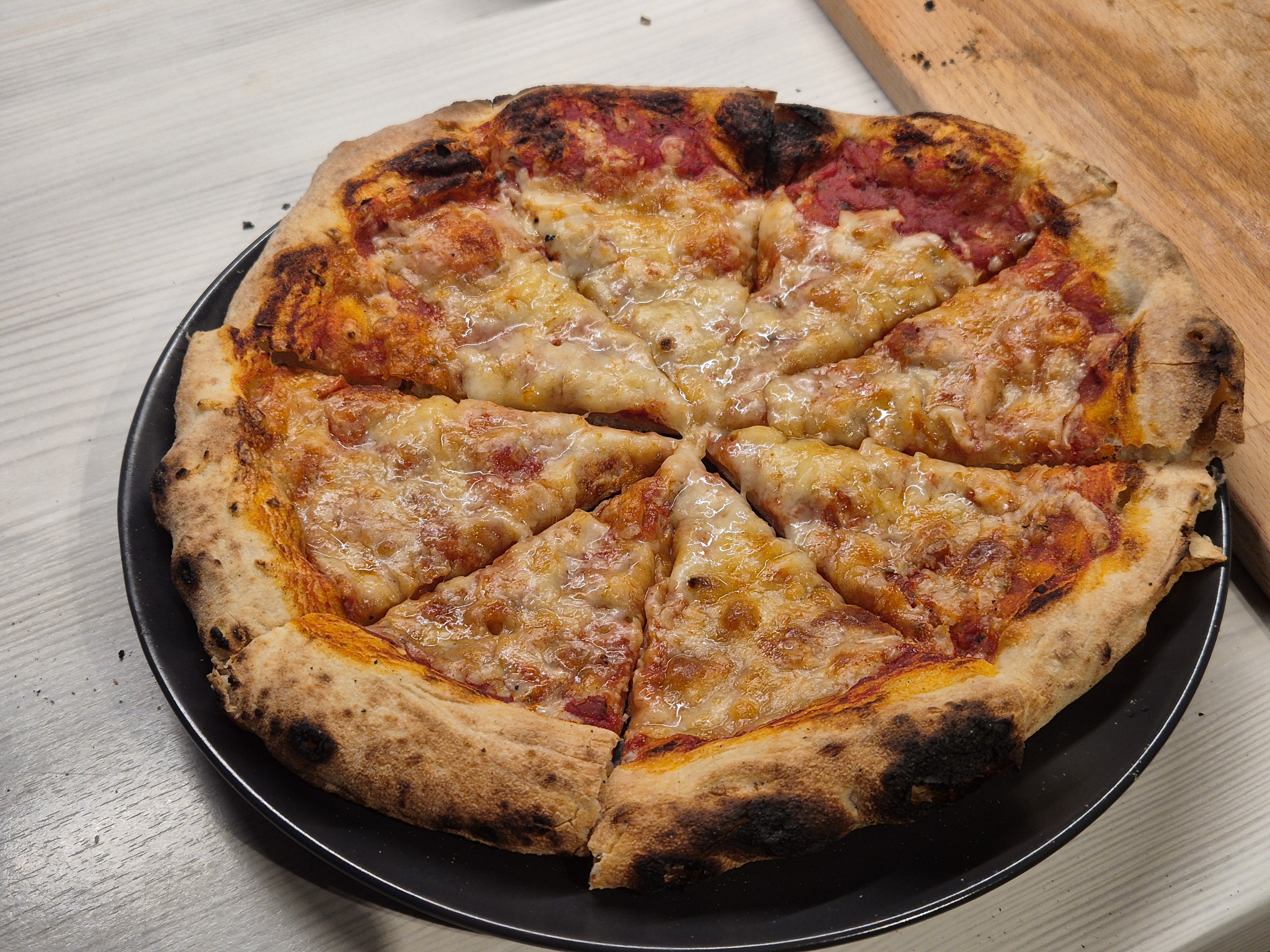
<p>After a few days in the freezer, it was the moment of the truth: I took a pizza out of the freezer, preheated the oven at 200°, and reheated for about 10 minutes.</p>

<p>All in all the pizza was delicious, but different than a fresh one by a mile. In particular the cheese on top was maybe a bit overcooked, and the crust was dry and crunchy in a slightly unpleasant way. So I would call it a success with a discrete margin of improvement.</p>

<div class="w3-row">
    <figure class="w3-col w3-center l6 m12 s12 blogpost-figure">
        <img src="/assets/images/blogposts/baking-frozen-pizza-from-scratch/first_attempt_packaged.jpg" alt="Frozen pizza straight out of the freezer." class="blogpost-image" />
        <figcaption class="caption blogpost-caption">Frozen pizza straight out of the freezer.</figcaption>
    </figure>

    <figure class="w3-col w3-center l6 m12 s12 blogpost-figure">
        <img src="/assets/images/blogposts/baking-frozen-pizza-from-scratch/first_attempt_completed.jpg" alt="Reheated pizza. The crust is noticeably dry and crumbly." class="blogpost-image" />
        <figcaption class="caption blogpost-caption">Reheated pizza. The crust is noticeably dry and crumbly.</figcaption>
    </figure>
</div>

<hr />

<h1 id="my-second-attempt">My second attempt</h1>

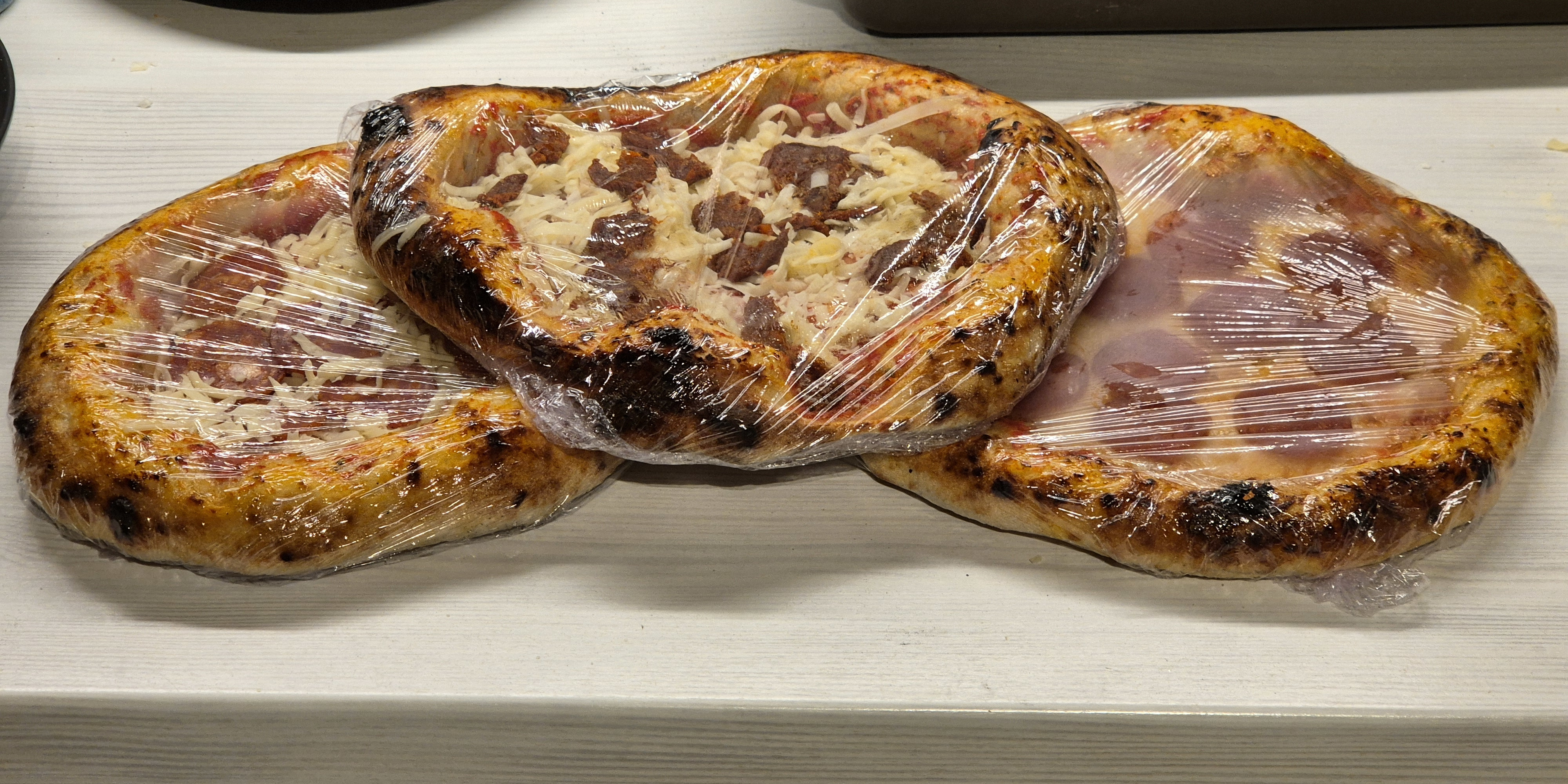
<p>For my second attempt I modified two steps in the procedure:</p>
<ul>
  <li>Tried swapping "Caputo Pizzeria" for "Caputo Nuvola";</li>
  <li>The toppings are now added AFTER an initial baking;</li>
  <li>Oil is added to the crust before freezing to prevent a dry crust.</li>
</ul>

<div class="w3-row">
    <figure class="w3-col w3-center l6 m12 s12 blogpost-figure">
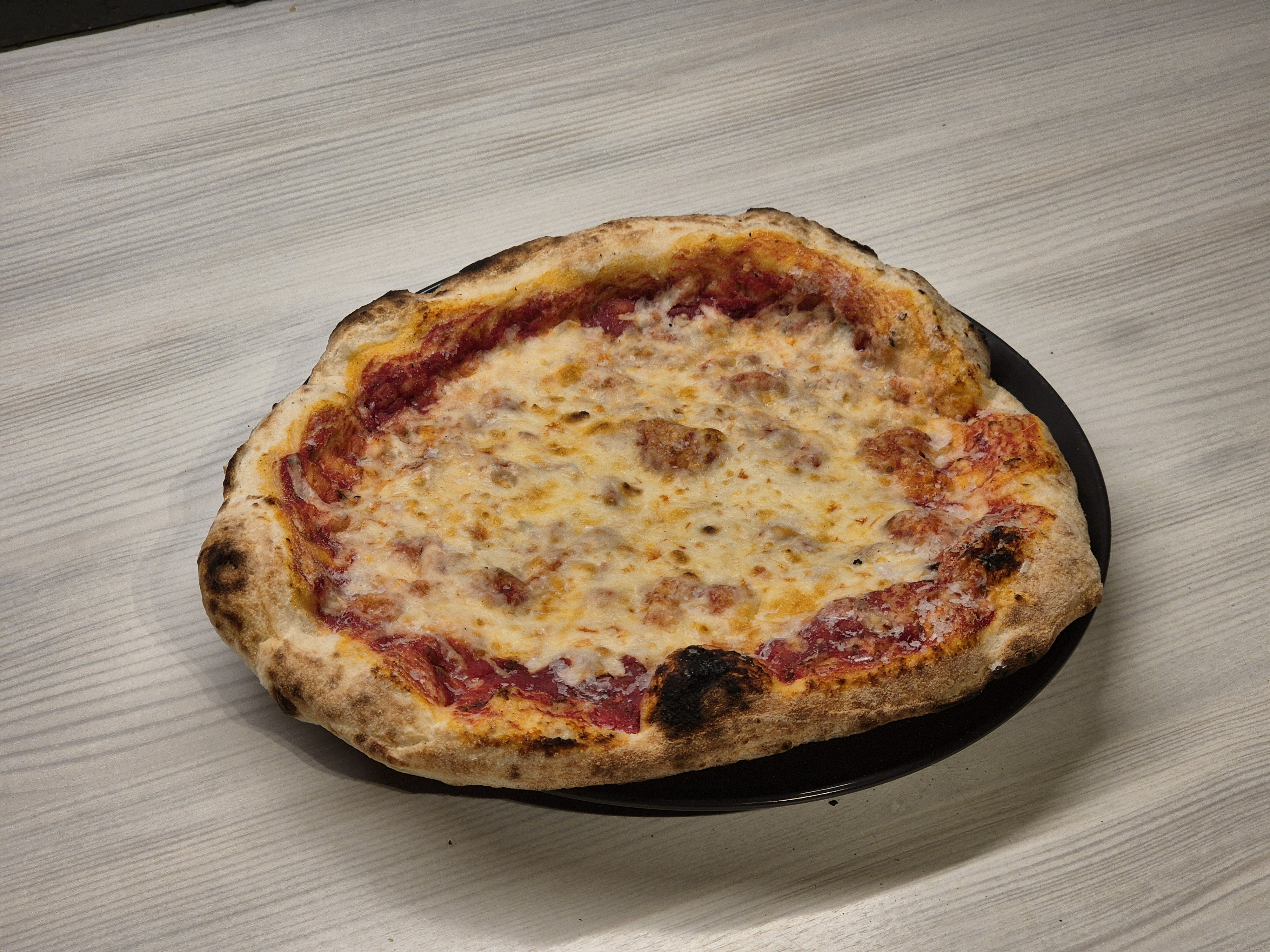
        <img src="/assets/images/blogposts/baking-frozen-pizza-from-scratch/second_attempt_packaged.jpg" alt="The final stack of pizzas prior to freezing." class="blogpost-image" />
        <figcaption class="caption blogpost-caption">The final stack of pizzas prior to freezing.</figcaption>
    </figure>

    <figure class="w3-col w3-center l6 m12 s12 blogpost-figure">
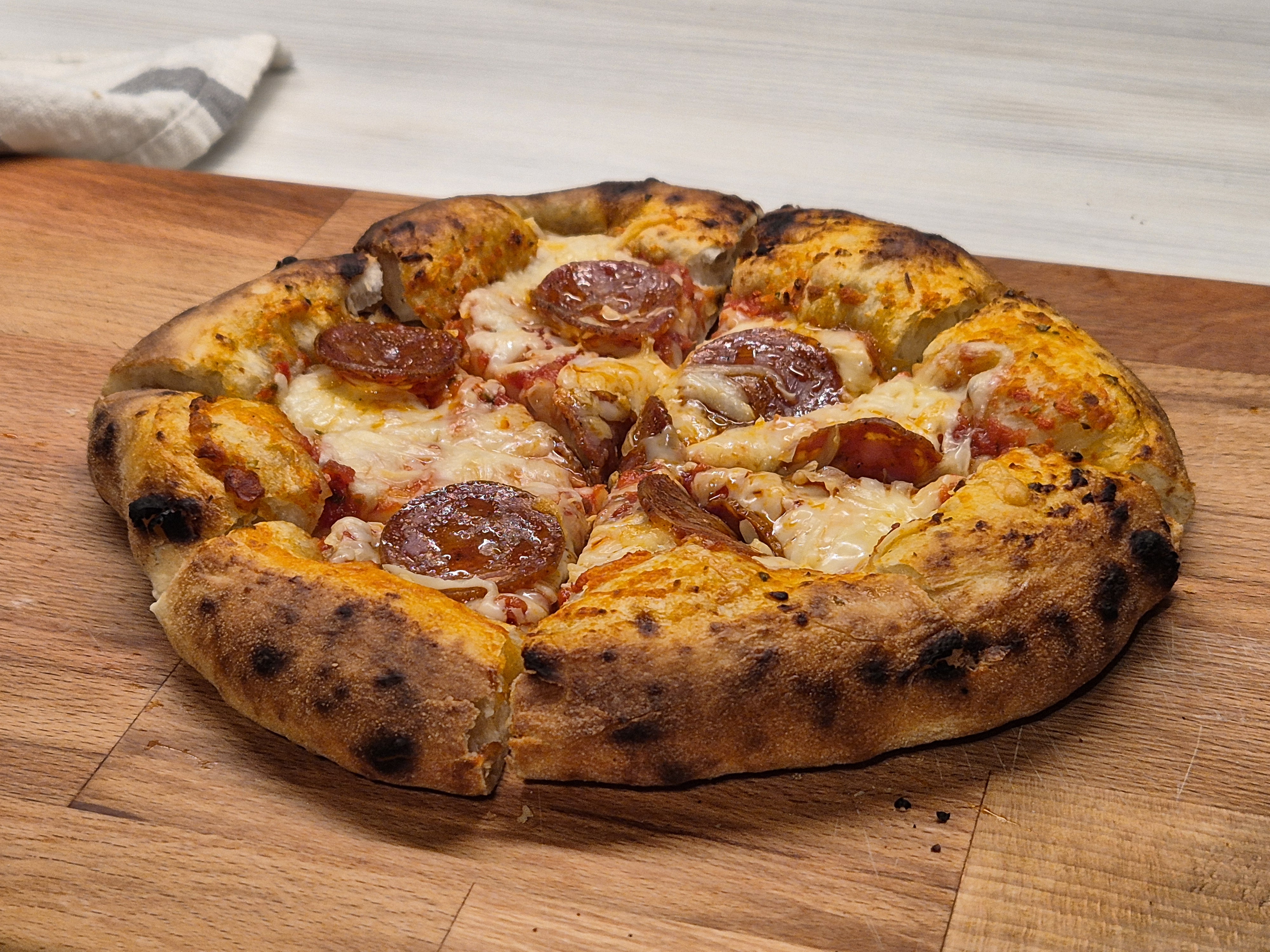
        <img src="/assets/images/blogposts/baking-frozen-pizza-from-scratch/second_attempt_sliced.jpg" alt="A second-batch pizza reheated." class="blogpost-image" />
        <figcaption class="caption blogpost-caption">A second-batch pizza reheated.</figcaption>
    </figure>
</div>

<p>These slight adjustments made a big difference. The pizza came out of the oven with cheese that was now hot but not "lava-like" hot, and the crust was less dry and crunchy, although still quite different from the fresh version.</p>

<p>The change of flour was not really noticeable.</p>

<hr />
<h1 id="conclusions">Conclusions</h1>

<p>When it comes to quality of the final product there is no comparison: the homemade frozen pizza beats the commercial ones hands down. Not only do they taste and feel better, but can be highly customizable allowing for a larger range of possibilities.</p>

<p>Let us now analyze the cost. To estimate it I will use the prices available to the retail customer in the Norwegian market as of November 2025.</p>

<p>Estimating the propane usage is not trivial, as it depends on the pre-heating time, the number of pizzas made per batch, and the speed of the pizzaiolo. By a back-of-the-envelope calculation I approximate a 5kg canister to be good for around 75 pizzas. Such a canister can be refilled completely for 269 NOK. Cost estimates assuming we are using all the ingredients in the most efficient way possible.</p>

<table>
  <thead>
    <tr>
      <th>Ingredient</th>
      <th>Quantity</th>
      <th>Cost per pizza (NOK)</th>
    </tr>
  </thead>
  <tbody>
    <tr>
      <td>Flour</td>
      <td>150 g</td>
      <td>6.19</td>
    </tr>
    <tr>
      <td>Water</td>
      <td>90 g</td>
      <td>0.00</td>
    </tr>
    <tr>
      <td>Oil</td>
      <td>5 g</td>
      <td>1.80</td>
    </tr>
    <tr>
      <td>Salt</td>
      <td>3.5 g</td>
      <td>&lt; 0.01</td>
    </tr>
    <tr>
      <td>Yeast</td>
      <td>0.75 g</td>
      <td>0.60</td>
    </tr>
    <tr>
      <td>Tomato sauce</td>
      <td>100 g</td>
      <td>1.80</td>
    </tr>
    <tr>
      <td>Cheese topping</td>
      <td>70 g</td>
      <td>9.63</td>
    </tr>
    <tr>
      <td>Gas</td>
      <td> </td>
      <td>3.60</td>
    </tr>
  </tbody>
  <tbody>
    <tr>
      <td><strong>Total</strong></td>
      <td> </td>
      <td><strong>23.62 NOK</strong></td>
    </tr>
  </tbody>
</table>

<p>Comparing it to the Norwegian national treasure <em>Grandiosa pizza</em> and the cheapest option <em>First Price margherita</em> — which sell at 59.90 NOK on <em>oda.no</em> and 29.90 NOK at the grocery chain <em>Meny</em> respectively — it seems like it pays off to bake homemade pizzas, also from a cost perspective.</p>

<h1 id="references">References</h1>

<div class="footnotes" role="doc-endnotes">
  <ol>
    <li id="fn:1">
      <p>Inoue, Y., and W. Bushuk. <em>“Studies on Frozen Doughs. II. Flour Quality Requirements for Bread Production from Frozen Dough.”</em> Cereal Chemistry, vol. 69, no. 4, 1992, pp. 423-428. <a href="#fnref:1" class="reversefootnote" role="doc-backlink">&#8617;</a></p>
    </li>
    <li id="fn:2">
      <p>Bárcenas, M. E., et al. <em>“Effect of freezing and frozen storage on the staling of part-baked and full-baked bread.”</em> <em>Journal of Food Engineering</em>, vol. 64, 2004, pp. 307–315. <a href="#fnref:2" class="reversefootnote" role="doc-backlink">&#8617;</a></p>
    </li>
  </ol>
</div>]]></content><author><name></name></author><category term="cooking" /><summary type="html"><![CDATA[At some point during one of my productive doomscrolling evenings, on YouTube specifically, I came across a video produced in November 2024 by Marcello Ascani featuring a pizzaiolo who moved to San Francisco, and was at the time working for a company producing Napolitan frozen pizzas in the Bay area.]]></summary><media:thumbnail xmlns:media="http://search.yahoo.com/mrss/" url="https://francesco.ballerin.it/assets/images/blogposts/baking-frozen-pizza-from-scratch/second_attempt_packaged.jpg" /><media:content medium="image" url="https://francesco.ballerin.it/assets/images/blogposts/baking-frozen-pizza-from-scratch/second_attempt_packaged.jpg" xmlns:media="http://search.yahoo.com/mrss/" /></entry><entry><title type="html">Map of aviation delays in Norway</title><link href="https://francesco.ballerin.it/2025/11/13/map-of-aviation-delays-norway.html" rel="alternate" type="text/html" title="Map of aviation delays in Norway" /><published>2025-11-13T00:00:00+00:00</published><updated>2025-11-13T00:00:00+00:00</updated><id>https://francesco.ballerin.it/2025/11/13/map-of-aviation-delays-norway</id><content type="html" xml:base="https://francesco.ballerin.it/2025/11/13/map-of-aviation-delays-norway.html"><![CDATA[<h1 id="motivation">Motivation</h1>

<p>Have you ever arrived at the airport, blissfully unaware, and suddenly found yourself submerged in chaos — a sea of people struggling with delays and cancellations? It is an absolute nightmare, and it happens to me regularly. To the extent that I have started looking up FlightRadar24 and Avinor's website to see what to expect prior to my arrival at the airport.</p>

<div class="w3-row">
    <figure class="w3-col w3-center l6 m12 s12 blogpost-figure">
        <img src="/assets/images/blogposts/map-of-aviation-delays-norway/cyberattack.png" alt="Reporting on the European cyberattack of September 2025 which caused several delays and cancellations in Europe. Courtesy of NRK [1]." class="blogpost-image" />
        <figcaption class="caption blogpost-caption">Reporting on the European cyberattack of September 2025 which caused several delays and cancellations in Europe. Courtesy of NRK [1].</figcaption>
    </figure>

    <figure class="w3-col w3-center l6 m12 s12 blogpost-figure">
        <img src="/assets/images/blogposts/map-of-aviation-delays-norway/chaos_drones.png" alt="Several hundred passengers stuck in Bergen due to delayed flights caused by drone sightings in Oslo. Courtesy of NRK [2]." class="blogpost-image" />
        <figcaption class="caption blogpost-caption">Several hundred passengers stuck in Bergen due to delayed flights caused by drone sightings in Oslo. Courtesy of NRK [2].</figcaption>
    </figure>
</div>

<p>I stumbled upon <a href="https://www.flightaware.com/miserymap/">FlightAware's Misery Map®</a> and got inspired; I decided to create something similar for the Norwegian airports, so that I can always know what to expect when heading to catch my next flight.</p>

<hr />

<h1 id="architecture">Architecture</h1>

<p>The architecture is fairly simple, and is based on <code class="language-plaintext highlighter-rouge">D3.js</code> for data visualization and <code class="language-plaintext highlighter-rouge">W3.CSS</code> for the stylesheet.</p>

<p>Avinor exposes a set of APIs that can be easily queried to obtain all the information we need to build the console. We just need a small middle layer to handle CORS requests, and possibly aggregate it so that we do not need to perform a request for every airport.</p>

<h3 id="avinor-apis">Avinor APIs</h3>

<p>The official API documentation can be found <a href="https://partner.avinor.no/tjenester/flydata/">here</a>, but I report here a brief summary of the query parameters and the response attributes.</p>

<h4 id="request">Request:</h4>

<table>
  <thead>
    <tr>
      <th>Parameter</th>
      <th>Description</th>
      <th>Example</th>
    </tr>
  </thead>
  <tbody>
    <tr>
      <td><code class="language-plaintext highlighter-rouge">airport</code></td>
      <td>IATA code of the airport of interest. Mandatory</td>
      <td><code class="language-plaintext highlighter-rouge">airport=OSL</code></td>
    </tr>
    <tr>
      <td><code class="language-plaintext highlighter-rouge">TimeFrom</code></td>
      <td>How many hours in the past to filter (positive, default=1)</td>
      <td><code class="language-plaintext highlighter-rouge">TimeFrom=2</code></td>
    </tr>
    <tr>
      <td><code class="language-plaintext highlighter-rouge">TimeTo</code></td>
      <td>How many hours in the future to filter (positive, default=7)</td>
      <td><code class="language-plaintext highlighter-rouge">TimeTo=5</code></td>
    </tr>
    <tr>
      <td><code class="language-plaintext highlighter-rouge">direction</code></td>
      <td>A=Arrivals, D=Departures, no value=both</td>
      <td><code class="language-plaintext highlighter-rouge">direction=D</code></td>
    </tr>
    <tr>
      <td><code class="language-plaintext highlighter-rouge">lastUpdate</code></td>
      <td>Load only flights that have been updated more recently than the specified time. Optional.</td>
      <td><code class="language-plaintext highlighter-rouge">lastUpdate=2024-08-08T09:30:00Z</code></td>
    </tr>
    <tr>
      <td><code class="language-plaintext highlighter-rouge">codeshare</code></td>
      <td>If included, also codeshare information is returned. Optional</td>
      <td><code class="language-plaintext highlighter-rouge">codeshare=Y</code></td>
    </tr>
    <tr>
      <td><code class="language-plaintext highlighter-rouge">serviceType</code></td>
      <td>E=include Helicopters, J=helicopters and service passengers, C=charters. default=only service passengers</td>
      <td><code class="language-plaintext highlighter-rouge">serviceType=E</code></td>
    </tr>
  </tbody>
</table>

<p>Notice that the request is airport-specific. Therefore, a request needs to be made for every single airport.</p>

<h4 id="response">Response:</h4>

<table>
  <thead>
    <tr>
      <th>Response</th>
      <th>Description</th>
      <th>Example</th>
    </tr>
  </thead>
  <tbody>
    <tr>
      <td><code class="language-plaintext highlighter-rouge">uniqueId</code></td>
      <td>Unique identifier. Max 12 numbers.</td>
      <td><code class="language-plaintext highlighter-rouge">1617049968</code></td>
    </tr>
    <tr>
      <td><code class="language-plaintext highlighter-rouge">lastUpdate</code></td>
      <td>Last update (edit) to the data</td>
      <td><code class="language-plaintext highlighter-rouge">2024-08-09T07:05:00Z</code></td>
    </tr>
    <tr>
      <td><code class="language-plaintext highlighter-rouge">flightId</code></td>
      <td>Flight codename</td>
      <td><code class="language-plaintext highlighter-rouge">SK4167</code></td>
    </tr>
    <tr>
      <td><code class="language-plaintext highlighter-rouge">dom_int</code></td>
      <td>D=domestic, S=Schengen, I=international</td>
      <td><code class="language-plaintext highlighter-rouge">D</code></td>
    </tr>
    <tr>
      <td><code class="language-plaintext highlighter-rouge">arr_dep</code></td>
      <td>A=arrival, D=departure</td>
      <td><code class="language-plaintext highlighter-rouge">D</code></td>
    </tr>
    <tr>
      <td><code class="language-plaintext highlighter-rouge">schedule_time</code></td>
      <td>Arrival/Departure scheduled time</td>
      <td><code class="language-plaintext highlighter-rouge">2024-08-09T07:05:00Z</code></td>
    </tr>
    <tr>
      <td><code class="language-plaintext highlighter-rouge">airport</code></td>
      <td>Arrival/Departure airport (the other airport)</td>
      <td><code class="language-plaintext highlighter-rouge">BGO</code></td>
    </tr>
    <tr>
      <td><code class="language-plaintext highlighter-rouge">airline</code></td>
      <td>IATA code of the airline</td>
      <td><code class="language-plaintext highlighter-rouge">SK</code></td>
    </tr>
    <tr>
      <td><code class="language-plaintext highlighter-rouge">via_airport</code></td>
      <td>Stops in IATA format, comma separated, max 10. Final destination not included</td>
      <td><code class="language-plaintext highlighter-rouge">SVG, BOO</code></td>
    </tr>
    <tr>
      <td><code class="language-plaintext highlighter-rouge">check_in</code></td>
      <td>Check-in area if provided</td>
      <td><code class="language-plaintext highlighter-rouge">1 2 3</code></td>
    </tr>
    <tr>
      <td><code class="language-plaintext highlighter-rouge">gate</code></td>
      <td>Gate if provided (departure only)</td>
      <td><code class="language-plaintext highlighter-rouge">B18</code></td>
    </tr>
    <tr>
      <td><code class="language-plaintext highlighter-rouge">belt_number</code></td>
      <td>Arrival belt if provided (arrival only)</td>
      <td><code class="language-plaintext highlighter-rouge">9</code></td>
    </tr>
    <tr>
      <td><code class="language-plaintext highlighter-rouge">status</code> <code class="language-plaintext highlighter-rouge">code</code></td>
      <td>A=arrived, C=Cancelled (or diverted), D=departed, E=new time, N=new info</td>
      <td><code class="language-plaintext highlighter-rouge">A</code></td>
    </tr>
    <tr>
      <td><code class="language-plaintext highlighter-rouge">status</code> <code class="language-plaintext highlighter-rouge">time</code></td>
      <td>Status time, relative to the code provided</td>
      <td><code class="language-plaintext highlighter-rouge">2024-08-09T07:05:00Z</code></td>
    </tr>
  </tbody>
</table>

<h3 id="cloudflare-workers">Cloudflare workers</h3>

<p>Cloudflare Workers are a serverless platform executing JavaScript snippets. Exactly what we need.</p>

<p>On the free plan we can process up to 100,000 requests a day, with a limitation on CPU time of 10 milliseconds per request.</p>

<p>Avinor's API is not configured for CORS requests, and therefore cannot handle direct-browser requests from arbitrary origins. The Worker fetches data from Avinor server-side, so the browser can safely call the Worker endpoint without running into CORS restrictions. Additionally, by the way the API is built, we need to query every single airport in Norway. Instead, I delegated this operation to the worker, who calls the API asynchronously and returns an aggregated result.</p>

<p>To reduce request volume to Avinor and make the UI faster, the Worker implements short-lived caching. The Worker sets appropriate Cache-Control headers and leverages the Cloudflare cache API to store JSON responses for a short TTL (in my case 60 seconds). This reduces API calls to Avinor while keeping data near real-time.</p>

<hr />

<h1 id="llm-usage">LLM usage</h1>

<p>Although I enjoy coding, especially if it is a data-driven project, I do not particularly enjoy UI-building and having to deal with HTML/CSS. JavaScript is also not my favorite programming language (clearly). So I took it as a good chance to see how far I could push agentic AI to help me build such a dashboard.</p>

<p>I knew already how I wanted to structure the project (<code class="language-plaintext highlighter-rouge">W3.CSS</code> + <code class="language-plaintext highlighter-rouge">D3.js</code> + Avinor's API + Cloudflare workers) so I described exactly how the API worked and what I wanted for a starting point and let the LLM do its magic.</p>

<p>The first result was usable but needing several BIG improvements. In particular:</p>
<ul>
  <li>
    <p>The agent tried to use the <a href="https://github.com/topojson/world-atlas">World Atlas TopoJSON</a> in the form of <code class="language-plaintext highlighter-rouge">countries-10m.json</code>, which was nowhere near fine enough for good visualization. I changed it to <code class="language-plaintext highlighter-rouge">countries-110m.json</code> and filtered the file to keep only the features for Norway to make requests lighter.</p>
  </li>
  <li>
    <p>The UI was there, but it was frankly quite terrible. The LLM tried to custom-make CSS code instead of using W3.CSS as instructed. But this was easily fixed.</p>
  </li>
  <li>
    <p>Although it had been fed the documentation on the API, it still applied the wrong logic to some of the data processing. For example, it mixed up departure and destination airports, and incorrectly classified cancelled flights.</p>
  </li>
  <li>
    <p>The default value for caching was set at 12s. I updated it to 60s, which is better but potentially still quite low.</p>
  </li>
</ul>

<p>Overall, it compressed the required workload from several days of painful UI-building to a few hours of high-level thinking and some debugging. So I am quite happy with this experiment.</p>

<p>Still, horizontal centering through CSS seems to be godly work that is beyond the capabilities of an LLM. Let's not talk about vertical centering.</p>

<hr />

<h1 id="future-developments">Future developments</h1>

<p>I would have loved to include a weather overlay, such as precipitation data coming from meteorological radars or nowcasting computed by the Norwegian Meteorological Institute. Unfortunately, I could not find such data for Norway readily available except as tiles that need to be processed and stitched together. I decided to leave it for another time.</p>

<p>I also thought the interactive visualization of the traffic streams on FlightAware's map was pretty cool, but that was way above my UI knowledge to implement and I did not dare asking the LLM to assist me with that. Maybe I will try to implement it at a later time.</p>

<h1 id="final-results-with-live-demo">Final results with live demo</h1>

<p>The live demo page can be found <a href="https://francesco.ballerin.it/norway_airports_map/">HERE</a>. Take a look at it!</p>

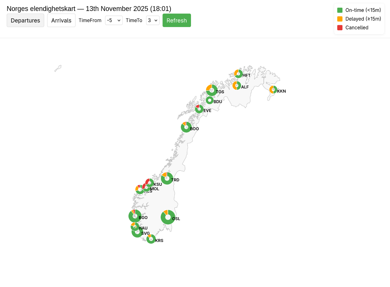
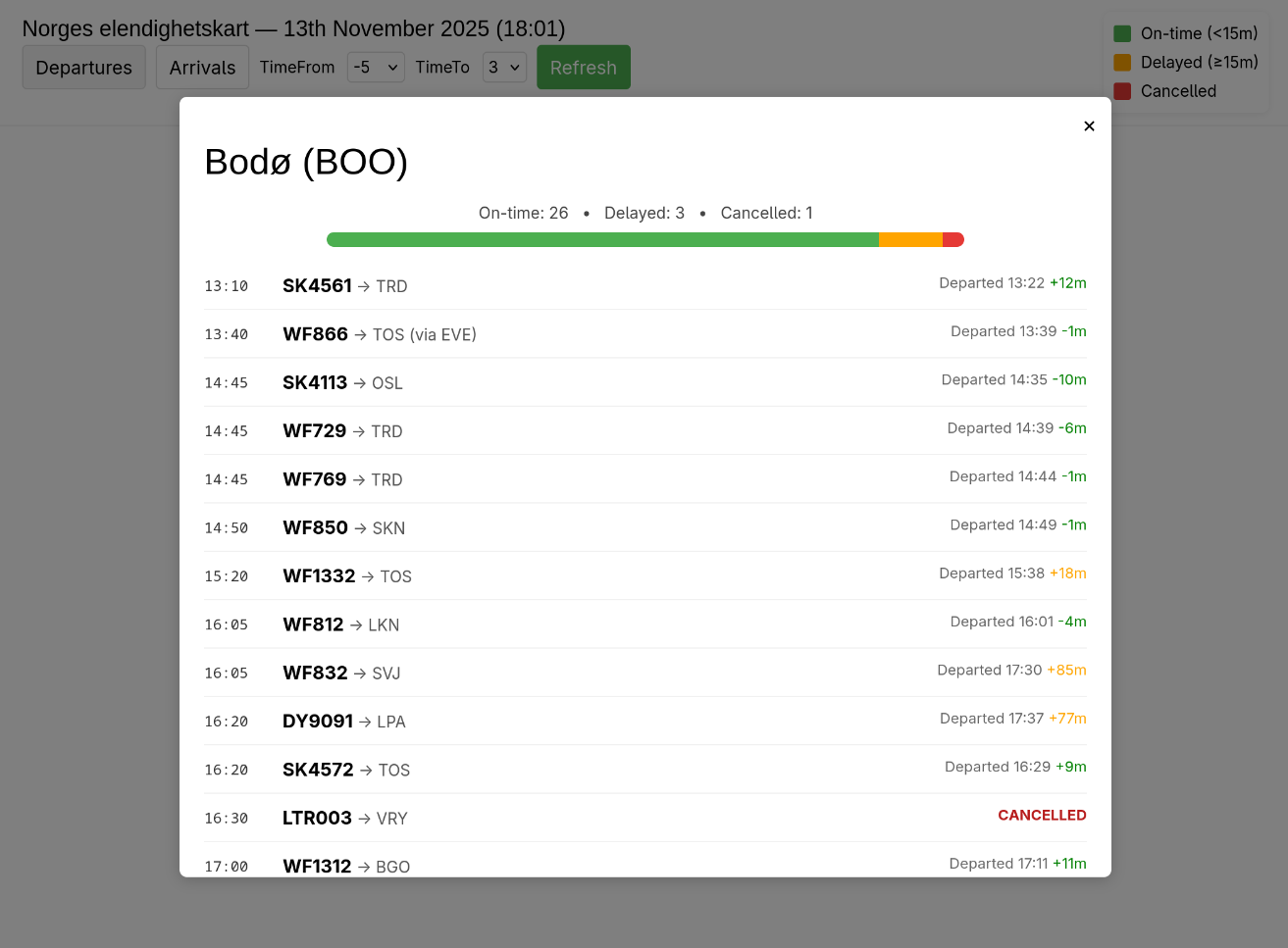
<p>Below are some screenshots.</p>

<div class="w3-row">
    <figure class="w3-col w3-center l6 m12 s12 blogpost-figure">
        <img src="/assets/images/blogposts/map-of-aviation-delays-norway/dashboard.png" alt="Main dashboard view." class="blogpost-image" />
        <figcaption class="caption blogpost-caption">Main dashboard view.</figcaption>
    </figure>

    <figure class="w3-col w3-center l6 m12 s12 blogpost-figure">
        <img src="/assets/images/blogposts/map-of-aviation-delays-norway/airport_detail.png" alt="Detailed view for a specific airport." class="blogpost-image" />
        <figcaption class="caption blogpost-caption">Detailed view for a specific airport.</figcaption>
    </figure>
</div>

<hr />

<h1 id="references">References</h1>
<p>[1]: <a href="https://www.nrk.no/urix/cyberangrep-mot-europeiske-flyplassar-1.17578597">https://www.nrk.no/urix/cyberangrep-mot-europeiske-flyplassar-1.17578597</a></p>

<p>[2]: <a href="https://www.nrk.no/vestland/flere-hundre-passasjerer-havnet-i-bergen-etter-droneobservasjoner-1.17582173">https://www.nrk.no/vestland/flere-hundre-passasjerer-havnet-i-bergen-etter-droneobservasjoner-1.17582173</a></p>]]></content><author><name></name></author><category term="projects" /><category term="data visualization" /><summary type="html"><![CDATA[I implemented a dashboard connected to Avinor to visualize the real-time air traffic state in Norway, with respect to delays and cancellations.]]></summary><media:thumbnail xmlns:media="http://search.yahoo.com/mrss/" url="https://francesco.ballerin.it/assets/images/blogposts/map-of-aviation-delays-norway/dashboard.png" /><media:content medium="image" url="https://francesco.ballerin.it/assets/images/blogposts/map-of-aviation-delays-norway/dashboard.png" xmlns:media="http://search.yahoo.com/mrss/" /></entry><entry><title type="html">RoboCup JR - Rescue Maze</title><link href="https://francesco.ballerin.it/2025/11/09/robocup-jr-2017.html" rel="alternate" type="text/html" title="RoboCup JR - Rescue Maze" /><published>2025-11-09T00:00:00+00:00</published><updated>2025-11-09T00:00:00+00:00</updated><id>https://francesco.ballerin.it/2025/11/09/robocup-jr-2017</id><content type="html" xml:base="https://francesco.ballerin.it/2025/11/09/robocup-jr-2017.html"><![CDATA[<h2 id="overview">Overview</h2>

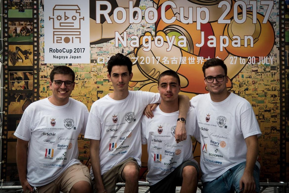
<p>In 2017 I participated, together with other three students from my high school — Daniele Gottardini, Alessandro Foradori, and Loris Gjini — to the international RoboCup JR competition which was held in Nagoya — Japan.</p>

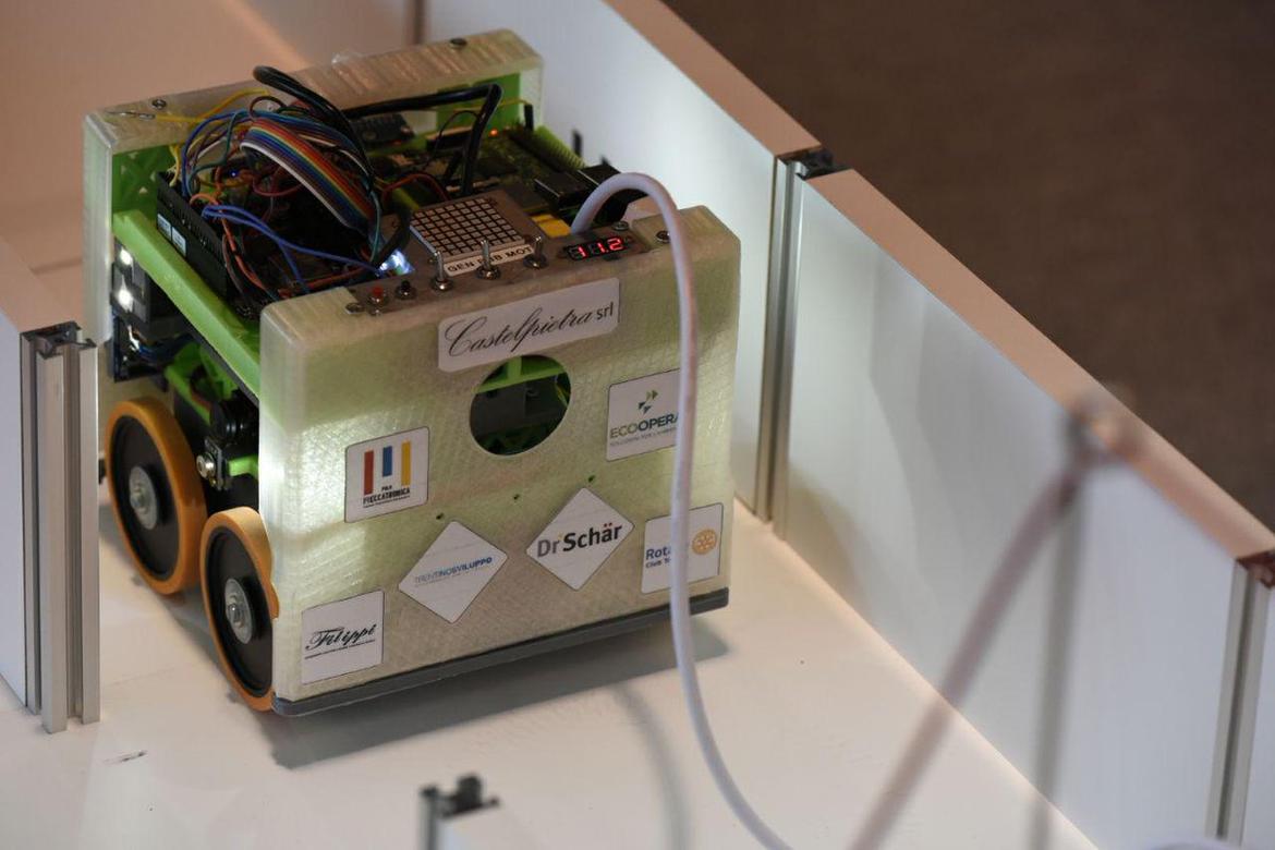
<div class="w3-row">
    <figure class="w3-col w3-center l12 m12 s12 blogpost-figure">
        <img src="/assets/images/blogposts/robocup-jr-2017/robot_in_maze.jpg" alt="The robot which we brought to Nagoya for the RoboCup JR International 2017." class="blogpost-image" />
        <figcaption class="caption blogpost-caption">The robot which we brought to Nagoya for the RoboCup JR International 2017.</figcaption>
    </figure>
</div>

<p>The motivation behind the competition was the simulation of an autonomous rescue effort in an unknown area which is considered too dangerous for human intervention. The rescue party (the robot) needs to be able to navigate the environment avoiding dangerous areas, navigating obstacles, searching for victims, and either rescuing the victims or dispensing rescue kits to them when found.</p>

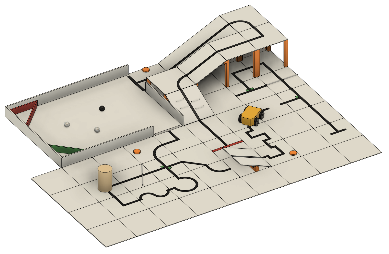
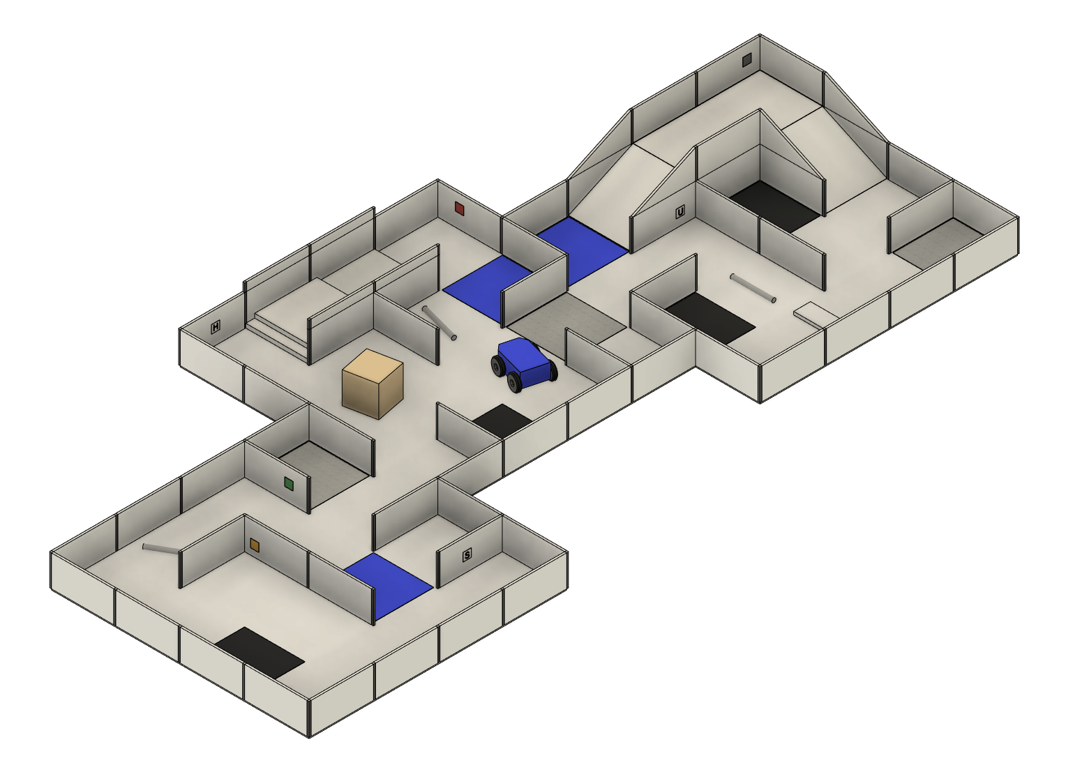
<p>The Rescue competitions were divided into two categories, for which every team is tasked to build from scratch an autonomous robot able to perform a certain number of actions. In <em>Rescue Line</em> the robot needs to follow a line, navigating intersections and obstacles, and ultimately move the victims to a safe location. In <em>Rescue Maze</em> the robot needs to explore a maze, avoid forbidden areas, navigate obstacles, and dispense rescue kits to the victims.</p>

<div class="w3-row">
    <figure class="w3-col w3-center l6 m12 s12 blogpost-figure">
        <img src="/assets/images/blogposts/robocup-jr-2017/rescue_line_arena.png" alt="Rescue Line arena." class="blogpost-image" />
        <figcaption class="caption blogpost-caption">Rescue Line arena.</figcaption>
    </figure>

    <figure class="w3-col w3-center l6 m12 s12 blogpost-figure">
        <img src="/assets/images/blogposts/robocup-jr-2017/rescue_maze_arena.png" alt="Rescue Maze arena." class="blogpost-image" />
        <figcaption class="caption blogpost-caption">Rescue Maze arena.</figcaption>
    </figure>
</div>

<hr />

<h2 id="background">Background</h2>

<p>While in high school I joined several extracurricular activities, among which my favorite one was probably the school's robotics club — a bunch of nerds hanging out once a week for a few hours, playing around with electronic components, 3D printing, and programming. The whole activity was organized under the supervision of Andrea Cristofori, a passionate lab technician who organized the whole thing and taking care of the "adult stuff" while enabling us to grow in an inspiring and stimulating environment.</p>

<p>The activities revolved around several projects, depending on the individual interests and needs of the participants. Some wanted to build small devices to automate repetitive tasks, others wanted to build their own drone from scratch, and some just wanted to tear down everyday consumer electronics devices to deeply understand their inner mechanisms. The main focus of the club was however the <em>RoboCup JR Italia</em> competition: a national competition taking place in the month of April or May each year, where teams from all around Italy meet up to compete in who is most capable in building an autonomous robot under a specific set of rules and constraints. The main prize is admission to the international level of the competition, and the honour to represent the country on the international stage.</p>

<p>During the school year we then devoted most of our efforts to designing and building a robot for the competition, learning valuable skills in the fields of 3D design and 3D printing, electronics, coding, and teamwork.</p>

<p>In the school year 2016–2017 we probably bit off more than we could chew in terms of ambition and decided to redesign the robot from scratch, leveraging experience from previous years. We sat down to brainstorm the solutions and design choices we wanted in our new build and designed the first iteration of what we eventually competed with at the national level.</p>

<p>The final result had to be a fully autonomous robot able to explore and map a maze, and ultimately find and "rescue" the victims. In the 2017 edition the maze was made of 30 cm × 30 cm tiles with potential walls on the sides. The floor surface was not smooth and could contain obstacles, bumpers, ramps, and small steps that the robot needed to navigate, making solid mechanics essential. The victims were located on the walls and were represented by one of two different features: either a heated pad that the robot needed to sense using a heat sensor, or a letter printed on the wall that needed to be recognized using a camera or some other "vision sensor".</p>

<hr />

<h2 id="our-robot">Our robot</h2>

<p>During our initial brainstorming we came up with many needs and wants, among which:</p>
<ul>
  <li>Linux-based project rather than microcontroller-based</li>
  <li>Efficient maze-exploring algorithms (Dijkstra's, BFS, A*, …)</li>
  <li>Custom diagnostic and monitoring tools with GUI</li>
  <li>Modular design with custom PCBs</li>
  <li>3D printed chassis with mechanical suspensions</li>
</ul>

<p>Let me go through these points one by one.</p>

<p>During the previous years we had experienced building robots based on Arduino, a simple open-source single-board microcontroller which can be programmed with its own programming language, which was close enough to C++ to make the learning curve not so steep, as C/C++ was part of the ordinary curriculum at our school. Arduino is an extremely cheap board, especially if using a Chinese knock-off version, which can take quite some beating without frying. It was perfect for learning the basics, but it had also many limitations. The biggest limitation, which we couldn't work past, was memory. It simply did not come with enough onboard memory to store the information of the maze and running our search algorithms. We discussed several solutions, among which using an SD card to store and retrieve bigger chunks of memory, but ultimately decided to just go for another board.</p>

<p>The popular Raspberry Pi board was very appealing, but it also came with its own set of limitations — notably the lack of real-time capabilities we needed to control some sensors and actuators. Looking back, we probably could have made it work by delegating the real-time tasks to an Arduino-based board, but at the time our eyes hovered over the BeagleBone Black boards: Linux-based boards with onboard Programmable Real-time Units (PRUs). Exactly what we needed.</p>

<p>Now that we had hardware capable enough to store all the information acquired about the maze in an appropriate data structure, we had to design our search-and-rescue algorithm. Ultimately, we opted for a simple algorithm that mixed a greedy approach with Dijkstra's algorithm. We represented the maze as a graph whose nodes are the Cartesian product of maze cells and the robot's possible states. Edges correspond to actions and are weighted by the time required to execute the movement and by the risk of getting stuck. Planning a path from one cell to another therefore meant running Dijkstra's algorithm to find the sequence of movements that minimized time and risk.</p>

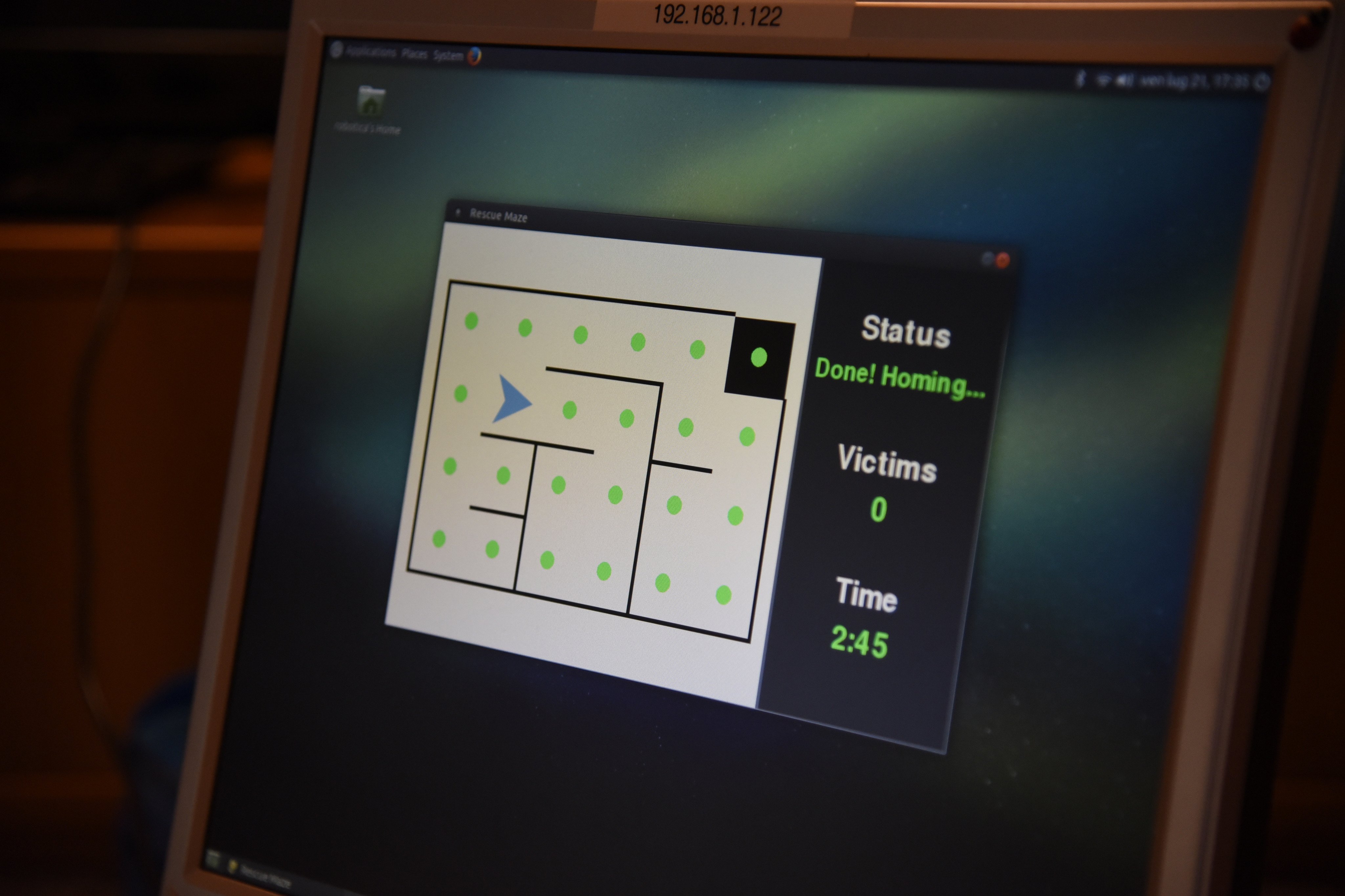
<p>This was easier said than done. Actually, after ironing out the bugs, implementing the algorithm was straightforward. In practice, however, running the algorithm based on our sensor data proved challenging due to varying sensitivity ranges and faulty readings. That required tweaking the graph weights and implementing a diagnostic tool to understand the fundamental issues.</p>

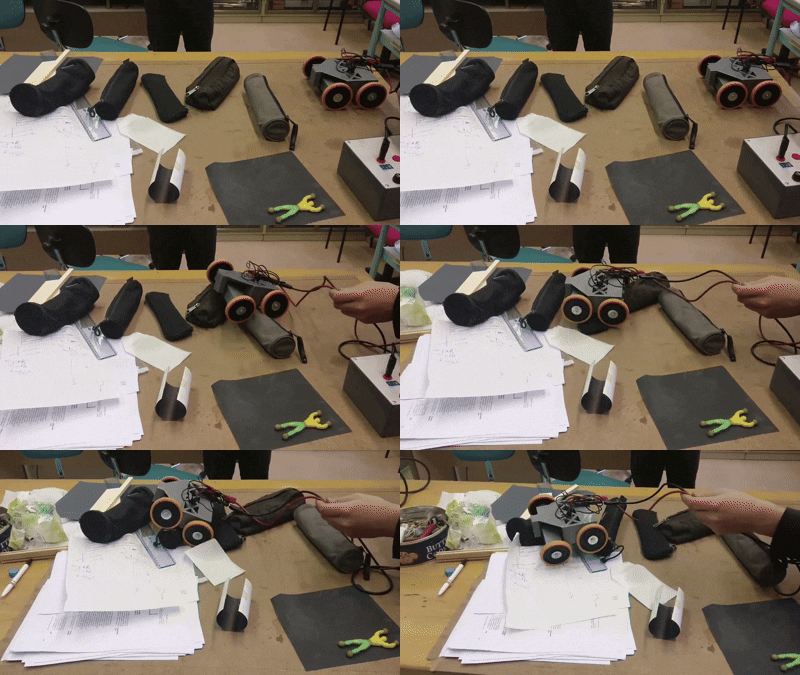
<p>On the physical design of the robot, Alessandro pushed really hard for a base with suspensions. Inspired by the design patterns on older farming equipment, he designed a pivoting system which required minimal maintenance and extra components. This design choice worked surprisingly well, and contributed in large part to the ability of the robot to navigate bumpers and debris without complicated software routines.</p>

<div class="w3-row">
    <figure class="w3-col w3-center l12 m12 s12 blogpost-figure">
        <img src="/assets/images/blogposts/robocup-jr-2017/suspensions.gif" alt="An early prototype of the base of the robot with our suspensions system." class="blogpost-image" />
        <figcaption class="caption blogpost-caption">An early prototype of the base of the robot with our suspensions system.</figcaption>
    </figure>
</div>

<p>To acquire the information coming from the sensors, logging, and diagnostics, we based our software on the Robot Operating System (ROS), which provided a plethora of tools specifically designed for robotics. We ended up using ROS only up to a small fraction of its full potential — the learning curve was steep and we were on a time crunch — but it proved extremely useful for handling sensor data and the communication between modules using the publisher/subscriber architecture. We implemented the debugging/diagnostic tool in Python, tapping into ROS's architecture, and built the GUI using the pygame library.</p>

<p>The computer-vision pipeline itself ran on the Raspberry Pi: the Pi handled camera capture and image processing (OpenCV) and sent recognition results to the BeagleBone Black over a simple serial link. We evaluated using a CNN approach, but ultimately opted for a lightweight preprocessing + k-nearest neighbors (KNN) classifier because it required far less training data and was easier to adapt to the real competition arenas for which we didn't have representative training examples.</p>

<div class="w3-row">
    <figure class="w3-col w3-center l6 m12 s12 blogpost-figure">
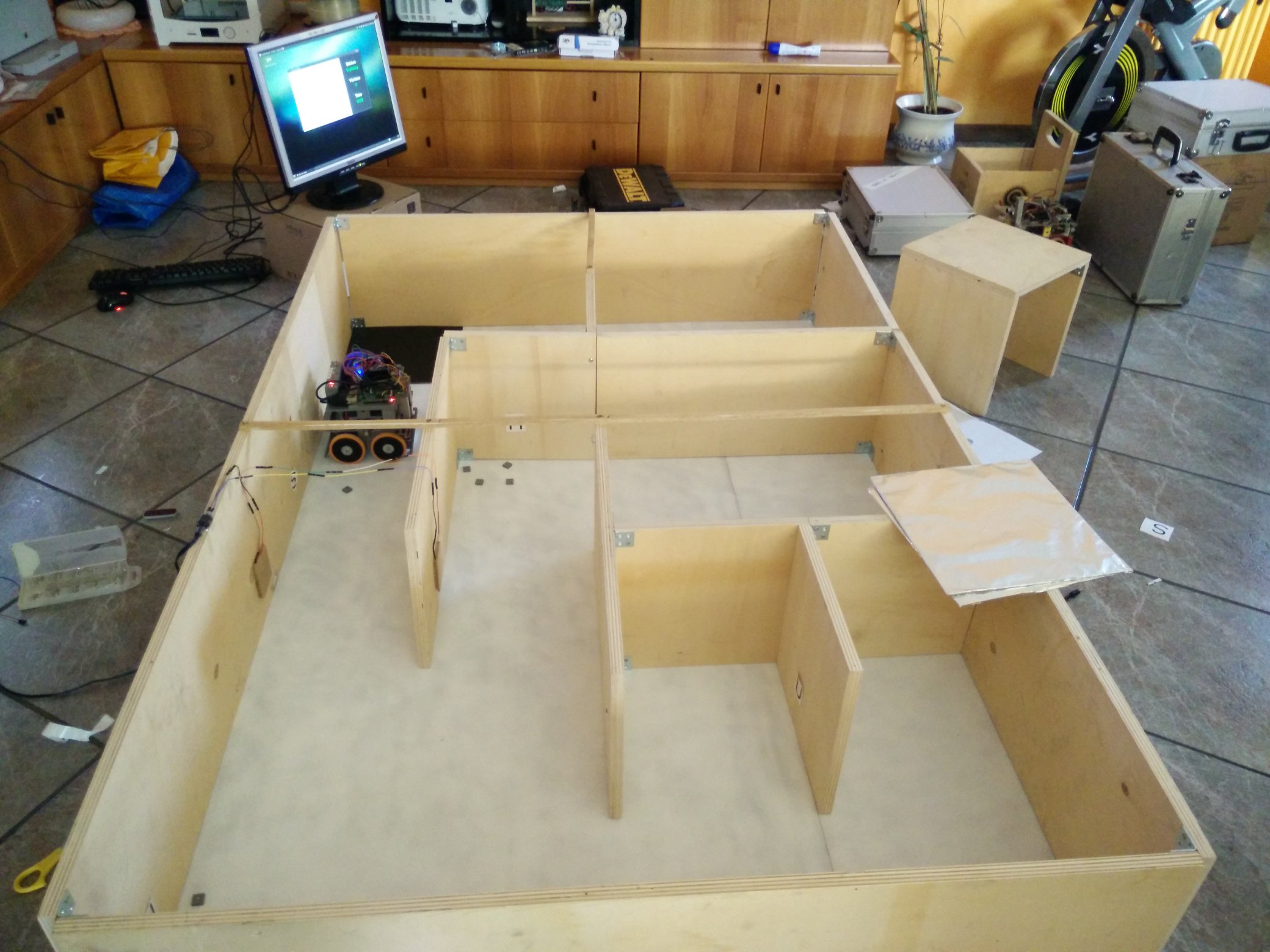
        <img src="/assets/images/blogposts/robocup-jr-2017/maze.gif" alt="Our robot navigating the maze (our testing arena) and successfully avoiding a prohibited zone (black tile)." class="blogpost-image" />
        <figcaption class="caption blogpost-caption">Our robot navigating the maze (our testing arena) and successfully avoiding a prohibited zone (black tile).</figcaption>
    </figure>

    <figure class="w3-col w3-center l6 m12 s12 blogpost-figure">
        <img src="/assets/images/blogposts/robocup-jr-2017/diagnostic_and_debug.jpg" alt="A shot of a monitor displaying one of the debugging tools we made. It ran real-time allowing us to understand if the robot's understanding of its environment was correct." class="blogpost-image" />
        <figcaption class="caption blogpost-caption">A shot of a monitor displaying one of the debugging tools we made. It ran real-time allowing us to understand if the robot's understanding of its environment was correct.</figcaption>
    </figure>
</div>

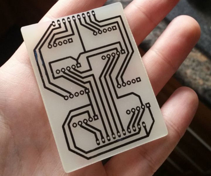
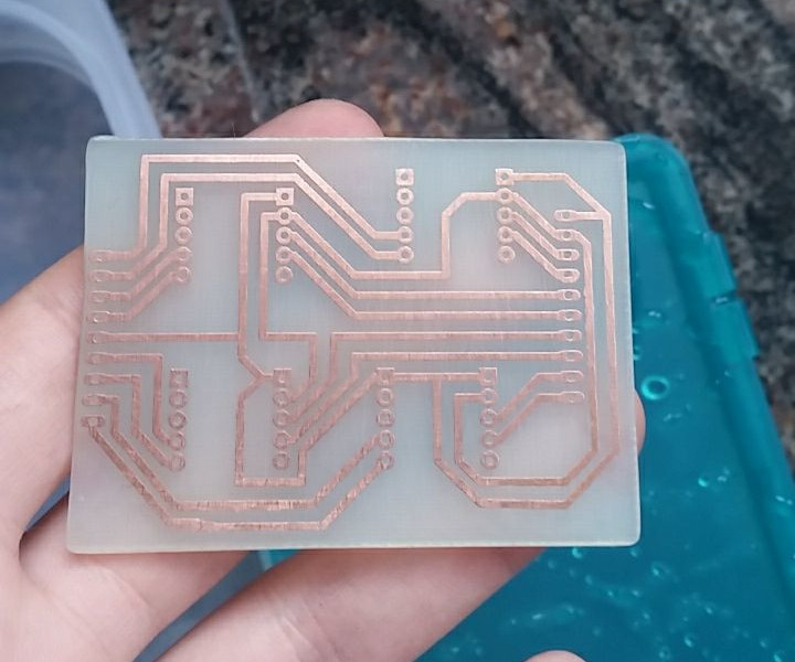
<p>To satisfy the requirement of modularity we decided to learn how to design and prototype PCBs using chemical etching. The process started with a blank copper-clad board and involved printing the PCB design with a laser printer onto regular paper and heat-transferring the toner lines onto the copper board. We then used an etching chemical such as ferric chloride to remove the excess copper not covered by the toner. The last step involved using acetone to remove the residual toner, leaving a clean finished board.</p>

<div class="w3-row">
    <figure class="w3-col w3-center l6 m12 s12 blogpost-figure">
        <img src="/assets/images/blogposts/robocup-jr-2017/pcb1.jpg" alt="Our custom sensors' PCB after etching." class="blogpost-image" />
        <figcaption class="caption blogpost-caption">Our custom sensors' PCB after etching.</figcaption>
    </figure>

    <figure class="w3-col w3-center l6 m12 s12 blogpost-figure">
        <img src="/assets/images/blogposts/robocup-jr-2017/pcb2.jpg" alt="The final product after polishing." class="blogpost-image" />
        <figcaption class="caption blogpost-caption">The final product after polishing.</figcaption>
    </figure>
</div>

<p>The specific components that were used for the robot were the following:</p>

<table>
  <thead>
    <tr>
      <th>Task</th>
      <th>Component</th>
      <th>Details</th>
    </tr>
  </thead>
  <tbody>
    <tr>
      <td>Main board</td>
      <td>BeagleBone Black version C</td>
      <td>Main logic, motor control</td>
    </tr>
    <tr>
      <td>Computer vision</td>
      <td>Raspberry Pi 2</td>
      <td>Running OpenCV</td>
    </tr>
    <tr>
      <td>Temperature sensor</td>
      <td>MLX90614</td>
      <td>For identifying the victims</td>
    </tr>
    <tr>
      <td>Distance sensor</td>
      <td>VL53L0X</td>
      <td>High-precision sensor — I2C</td>
    </tr>
    <tr>
      <td>Distance sensor</td>
      <td>HC-SR04</td>
      <td>Backup sensor with low precision — PWM</td>
    </tr>
    <tr>
      <td>Color sensor</td>
      <td>TCS34725</td>
      <td>For recognizing and avoiding the black tiles — I2C</td>
    </tr>
    <tr>
      <td>Orientation sensor</td>
      <td>MPU-6050</td>
      <td>Serial communication</td>
    </tr>
    <tr>
      <td>Camera</td>
      <td>USB100W03M</td>
      <td>USB — connected to Raspi</td>
    </tr>
    <tr>
      <td>DC motors</td>
      <td>Maxon</td>
      <td>PWM</td>
    </tr>
    <tr>
      <td>Rescue kit dispenser</td>
      <td>Servo 9g</td>
      <td>PWM</td>
    </tr>
  </tbody>
</table>

<p>The main upgrade for which we were most excited was the use of Time-of-Flight (ToF) distance sensors. A ToF sensor measures how long it takes for an emitted infrared laser pulse to reflect back from a target, giving much more precise distance readings compared to an HC-SR04 ultrasonic distance sensor. It features two modes: a <em>single-shot mode</em>, which produces a measurement on demand, and a <em>continuous mode</em>, which measures the distance at regular intervals (commonly on the order of 100 ms).</p>

<p>As I mentioned, this turned out to be more than we could chew. Or more precisely — we managed to build the robot in time for the competition, but the amount of testing that we managed to perform before the competition was minimal. This in turn caused many bugs to be left in the final product.</p>

<hr />

<h2 id="the-national-competition-in-foligno-and-the-european-competition-in-montesilvano">The national competition in Foligno and the European competition in Montesilvano</h2>

<p>The 2017 national competition was organized in the town of Foligno.</p>

<p>I will cut this short: we did not win this competition. The lack of testing showed itself clearly, and specifically in the form of sensors issues.</p>

<p>The VL53L0X Time-of-Flight distance sensors, in which we had high expectations, ended up failing us. It was not the sensors themselves but rather the high-level library we used to manage them. That library — the only high-level Python library available at the time — could only read the sensors in single-shot mode using a blocking procedure. The BeagleBone's I2C interface therefore could not handle multiple readings in parallel, and each reading was slow. Okay — each reading was only a few hundred milliseconds, but because we had 12 sensors in total the delay became critical.</p>

<p>Although this was not the only bug, it was certainly the main one. During the competition days we mitigated it by reducing the number of active sensors while the robot was moving and by prioritizing those directed toward the front. This, however, reduced precision and left the robot overall slow-moving.</p>

<p>Ultimately, we did not perform too badly at the competition. But the early rounds impacted the overall score, and ultimately we did not make it to the podium.</p>

<div class="w3-row">
    <figure class="w3-col w3-center l6 m12 s12 blogpost-figure">
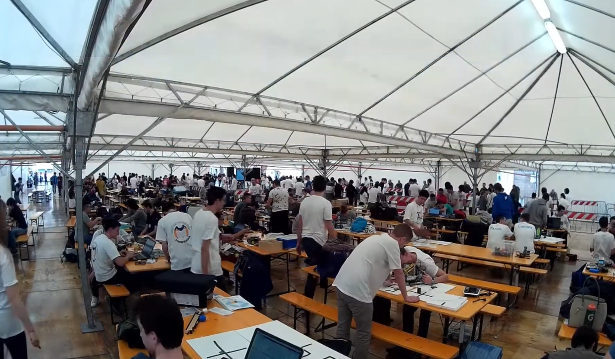
        <img src="/assets/images/blogposts/robocup-jr-2017/foligno_venue.png" alt="The venue of the competitions in Foligno." class="blogpost-image" />
        <figcaption class="caption blogpost-caption">The venue of the competitions in Foligno.</figcaption>
    </figure>

    <figure class="w3-col w3-center l6 m12 s12 blogpost-figure">
        <img src="/assets/images/blogposts/robocup-jr-2017/foligno_arena.jpg" alt="The Rescue Maze arena used in Foligno." class="blogpost-image" />
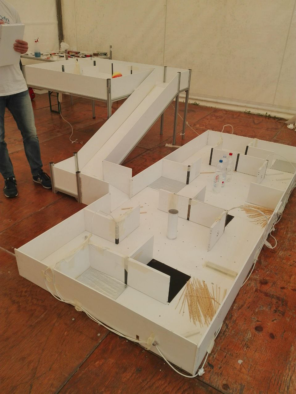
        <figcaption class="caption blogpost-caption">The Rescue Maze arena used in Foligno.</figcaption>
    </figure>
</div>

<p>A new occasion presented itself in the form of the European competition in Montesilvano (Pescara). This was a European-level competition (SuperRegional competition) which served as a middle-ground between the regional/national competitions and the main international one.</p>

<p>With one extra month to mitigate the issues we faced, we greatly improved on the leaderboard, finishing in second place — just behind the Croatian team, which had already qualified for the international level from their national competition (and which — spoiler — went on to win the world title in Japan).</p>

<p>Unfortunately, the European competition did not grant automatic qualification to the international level, but only on the condition that any spot became available due to excess capacity of the international venue, or any of the other teams dropped out.</p>

<p>For the month following the Montesilvano competition we had intense correspondence with the international organization to see if a spot would become available, and eventually we received positive feedback.</p>

<p>It was now time to prepare for the next step: Japan.</p>

<hr />

<h2 id="the-international-competition-in-nagoya-japan">The international competition in Nagoya, Japan</h2>

<p>Excited at the prospect of competing in Japan and representing Italy on the international stage (together with the other Italian team from Schio, which had qualified in Foligno), we started working again on the robot.</p>

<p>Only two obstacles stood between us and the trip. 2017 was our graduation year, and finals took place in June and early July. As soon as the exams were over, the school would close for the summer.</p>

<p>There was no way around the first issue: we had to split our time between graduation and the robot until the end of the finals. After the school shut down we moved into my parents' house in Strigno and brought with us half of the lab.</p>

<div class="w3-row">
    <figure class="w3-col w3-center l6 m12 s12 blogpost-figure">
        <img src="/assets/images/blogposts/robocup-jr-2017/livingroom.jpg" alt="The state of my parents' livingroom for the whole summer prior to the competition (my mother is a very patient woman)." class="blogpost-image" />
        <figcaption class="caption blogpost-caption">The state of my parents' livingroom for the whole summer prior to the competition (my mother is a very patient woman).</figcaption>
    </figure>

    <figure class="w3-col w3-center l6 m12 s12 blogpost-figure">
        <img src="/assets/images/blogposts/robocup-jr-2017/robot_work_in_progress.jpg" alt="Daniele upgrading one of the modules. On the right, the front panel of the robot with the logos of our generous sponsors." class="blogpost-image" />
        <figcaption class="caption blogpost-caption">Daniele upgrading one of the modules. On the right, the front panel of the robot with the logos of our generous sponsors.</figcaption>
    </figure>
</div>

<p>In Strigno we spent a few very intense weeks: on the one hand upgrading the hardware and software, ironing out bugs and performing as many test rounds as possible; on the other hand seeking sponsors to cover the participation fees and travel costs. After all, a trip to Japan did not come cheap, especially in summer, and the school had very little disposable budget for this type of activity following many years of cuts in public funding.</p>

<p>Over the summer we managed to find several generous local companies whose contributions allowed us to go to Japan. In no particular order these were:</p>
<ul>
  <li>Castelpietra S.r.l. — specializing in measurement tools in the automotive industry;</li>
  <li>Polo meccatronica — technology hub in Rovereto;</li>
  <li>Ecoopera — waste management solutions;</li>
  <li>TrentinoSviluppo — local agency for innovation, business, and territorial development for the Trentino province;</li>
  <li>Filippi — a family-run confectionery shop in Trento;</li>
  <li>Dr Schär — leader in production of gluten-free foods and snacks;</li>
  <li>Rotary Club Trento — the regional division of the Rotary Club International.</li>
</ul>

<div class="w3-row">
    <figure class="w3-col w3-center l4 m12 s12 blogpost-figure">
        <img src="/assets/images/blogposts/robocup-jr-2017/nagoya_map.jpg" alt="Loris and Daniele figuring the way from the airport to the hotel." class="blogpost-image" />
        <figcaption class="caption blogpost-caption">Loris and Daniele figuring the way from the airport to the hotel.</figcaption>
    </figure>

    <figure class="w3-col w3-center l4 m12 s12 blogpost-figure">
        <img src="/assets/images/blogposts/robocup-jr-2017/working_hard.jpg" alt="From the left Alessandro, Daniele, and myself." class="blogpost-image" />
        <figcaption class="caption blogpost-caption">From the left Alessandro, Daniele, and myself.</figcaption>
    </figure>

    <figure class="w3-col w3-center l4 m12 s12 blogpost-figure">
        <img src="/assets/images/blogposts/robocup-jr-2017/competition.jpg" alt="Alessandro and I during one of the rounds." class="blogpost-image" />
        <figcaption class="caption blogpost-caption">Alessandro and I during one of the rounds.</figcaption>
    </figure>
</div>

<p>The competition rounds were split among two days for the main competition, with an extra day for the "SuperTeam": two teams from different countries were randomly matched in order to coordinate and compete against the other pairs in a new competition that was kept secret until the days of the event. With such short notice, the aim of this new competition was to test the ability to adapt and problem-solve in an extreme time crunch, as well as to work around language and cultural barriers.</p>

<p>During the competition days, technical interviews also took place to award the following additional prizes:</p>
<ul>
  <li>Best Software Programming</li>
  <li>Best Rescue Engineering Strategy</li>
  <li>Best Innovation</li>
  <li>Best Presentation</li>
  <li>Best Team Spirit</li>
</ul>

<div class="w3-row">
    <figure class="w3-col w3-center l4 m12 s12 blogpost-figure">
        <img src="/assets/images/blogposts/robocup-jr-2017/comp_robot_1.jpg" alt="One of the other participating teams. Flying wiring was a very popular design choice." class="blogpost-image" />
        <figcaption class="caption blogpost-caption">One of the other participating teams. Flying wiring was a very popular design choice.</figcaption>
    </figure>

    <figure class="w3-col w3-center l4 m12 s12 blogpost-figure">
        <img src="/assets/images/blogposts/robocup-jr-2017/comp_robot_2.jpg" alt="The robot of the Australian team, featuring a full LIDAR system." class="blogpost-image" />
        <figcaption class="caption blogpost-caption">The robot of the Australian team, featuring a full LIDAR system.</figcaption>
    </figure>

    <figure class="w3-col w3-center l4 m12 s12 blogpost-figure">
        <img src="/assets/images/blogposts/robocup-jr-2017/comp_robot_3.jpg" alt="The robot of the Mexican team, built with laser cut panels." class="blogpost-image" />
        <figcaption class="caption blogpost-caption">The robot of the Mexican team, built with laser cut panels.</figcaption>
    </figure>
</div>

<p>Although our robot had many bugs resolved and the software had become more reliable, we ultimately didn't qualify for the podium and finished around the middle of the leaderboard. Considering this was the international level of the competition, which saw the best teams from all over the world competing for a spot on the podium, this was in no way a trivial achievement.</p>

<p>For the SuperTeam we were paired with a Chinese team and given very little time to coordinate. We started by showing each other the high-level parts of our systems — their sensors and control heuristics and our mapping and path-planning routines — and agreed on a minimal interface so the two stacks could interoperate for the collaboartive run. Thankfully, we had brought with us a couple of bluetooth serial chips that we could use to connect the two robots. Communication was challenging at first (language and cultural differences), so we relied heavily on sketches and Google Translate. The resulting cooperation was imperfect but effective — we managed to place ourselves again around the middle of the leaderboard.</p>

<p>Shortly before the award ceremony, the jury informed us that our team had won the <em>Best Software Programming</em> prize. The award felt especially meaningful to us: the judges explicitly cited our computer vision letter-recognition algorithm and the ROS integration as key reasons for the decision, and we were genuinely delighted and proud to receive it.</p>

<div class="w3-row">
    <figure class="w3-col w3-center l6 m12 s12 blogpost-figure">
        <img src="/assets/images/blogposts/robocup-jr-2017/team.jpg" alt="The team in front of the venue." class="blogpost-image" />
        <figcaption class="caption blogpost-caption">The team in front of the venue.</figcaption>
    </figure>

    <figure class="w3-col w3-center l6 m12 s12 blogpost-figure">
        <img src="/assets/images/blogposts/robocup-jr-2017/award.jpg" alt="Award for Best Software, on top of my now retired XPS 9560." class="blogpost-image" />
        <figcaption class="caption blogpost-caption">Award for Best Software, on top of my now retired XPS 9560.</figcaption>
    </figure>
</div>

<hr />

<h2 id="takeaways-and-considerations">Takeaways and considerations</h2>

<p>This project left us with lessons that reach far beyond the technical stack. Building a competition robot forced us to make choices every day about what to prioritize, how to split effort, and how to persist when things broke in unexpected ways. Time management proved as important as code: we learned to break large problems into small, testable goals, to schedule focused blocks of work around exams and other obligations, and to accept that shipping imperfect but well-tested features is often better than waiting for perfection.</p>

<p>Teamwork was the engine that made everything possible. Each member brought different strengths — mechanics, electronics, algorithms, or a calm head in a crisis — and trusting one another to own pieces of the project let us move faster than any of us could alone. We learned to communicate more clearly and to ask for help early when in need. When something failed on the field, we debugged together: someone watched logs and tried software patches, another inspected wiring and sensors. Those moments taught us resilience, how to divide responsibility, and how to turn mistakes into learning opportunities.</p>

<p>Finally, competing internationally was a gentle reminder that engineering is also a cultural exchange. In Nagoya we met teams from other countries, each with different approaches, tools, and ways of approaching problems. Conversations over coffee (or charging LiPo batteries) or in the pit area expanded our toolkit and our perspective. Teamwork with the Chinese team in preparation of the Superteam challenge, dealing with a tall language and cultural barrier, was an enriching experience and one of our first true international collaborations.</p>

<p>Many lessons were learned along the way, and although the engineering aspects are the most evident in a project like this, I am not sure they were more valuable or enriching than the lessons in time management, PR and sponsors acquisition, humility, and teamwork.</p>

<hr />

<h2 id="acknowledgments">Acknowledgments</h2>

<p>I would like to dedicate this blogpost to two key people in our journey: Andrea Cristofori and Fredrik Löfgren. Andrea was for us a great mentor, who selflessly dedicated a gargantuan amount of time and effort to the school and to us without ever asking for anything in return. Without him there would not have been a robotics club at all. Fredrik was a great judge and organizer, always available and friendly. He supported our participation in the international RoboCup JR competition and promptly helped us with the application process once a spot opened up after the European SuperRegional competition.</p>

<p>Unfortunately, Fredrik tragically passed away in 2024 in an accident involving a bus in Stockholm. He is fondly remembered by all of us.</p>

<div class="w3-row">
    <figure class="w3-col w3-center l6 m12 s12 blogpost-figure">
        <img src="/assets/images/blogposts/robocup-jr-2017/cristofori.jpg" alt="Andrea Cristofori in Nagoya, directing us from the hotel to the venue." class="blogpost-image" />
        <figcaption class="caption blogpost-caption">Andrea Cristofori in Nagoya, directing us from the hotel to the venue.</figcaption>
    </figure>

    <figure class="w3-col w3-center l6 m12 s12 blogpost-figure">
        <img src="/assets/images/blogposts/robocup-jr-2017/fredrik.jpg" alt="Fredrik Löfgren at the venue in Nagoya." class="blogpost-image" />
        <figcaption class="caption blogpost-caption">Fredrik Löfgren at the venue in Nagoya.</figcaption>
    </figure>
</div>]]></content><author><name></name></author><category term="projects" /><category term="robotics" /><summary type="html"><![CDATA[In 2017 I participated in the RoboCup JR competition in Nagoya — Japan — developing a robot able to navigate a maze and perform certain tasks autonomously, based on BeagleBone and Raspberry Pi]]></summary><media:thumbnail xmlns:media="http://search.yahoo.com/mrss/" url="https://francesco.ballerin.it/assets/images/blogposts/robocup-jr-2017/robot_in_maze.jpg" /><media:content medium="image" url="https://francesco.ballerin.it/assets/images/blogposts/robocup-jr-2017/robot_in_maze.jpg" xmlns:media="http://search.yahoo.com/mrss/" /></entry><entry><title type="html">Why I started a blog in 2025 (and why you should consider it too)</title><link href="https://francesco.ballerin.it/2025/10/17/why-I-started-a-blog-in-2025.html" rel="alternate" type="text/html" title="Why I started a blog in 2025 (and why you should consider it too)" /><published>2025-10-17T00:00:00+00:00</published><updated>2025-10-17T00:00:00+00:00</updated><id>https://francesco.ballerin.it/2025/10/17/why-I-started-a-blog-in-2025</id><content type="html" xml:base="https://francesco.ballerin.it/2025/10/17/why-I-started-a-blog-in-2025.html"><![CDATA[<p>I have decided to start a blog — about everything and nothing in particular. This has been a project I have been thinking about for quite a long time, and there are many reasons that finally pushed me to cave in and throw myself at it. Mainly, though, I am doing it for myself.</p>

<p>I have always been drawn to new side projects and hobbies — ways to express ideas and creativity that otherwise are left to sit and seethe in a corner of my mind, desperately calling and begging to be let out.</p>

<p>Since I moved in 2019 from Trento (Italy) to Bergen (Norway), I have picked up many different new hobbies, and gave it a go to several side projects. Sometimes they were motivated by a need — learning to cook Italian dishes after moving abroad, starting to brew beer to have cheap, delicious beer, or studying nutrition and training to start a journey into a healthier life — and other times they were pure curiosity, like trying oil painting à la Bob Ross, photography, or woodworking.</p>

<div class="w3-row">
    <figure class="w3-col w3-center l6 m12 s12 blogpost-figure">
        <img src="/assets/images/blogposts/why-I-started-a-blog-in-2025/ballerinus_apple_cider.jpg" alt="A production of Apple Cider, with custom labels" class="blogpost-image" />
        <figcaption class="caption blogpost-caption">A production of Apple Cider, with custom labels</figcaption>
    </figure>

    <figure class="w3-col w3-center l6 m12 s12 blogpost-figure">
        <img src="/assets/images/blogposts/why-I-started-a-blog-in-2025/second_bob_ross_painting.jpg" alt="My second ever attempt at a Bob Ross-inspired oil painting" class="blogpost-image" />
        <figcaption class="caption blogpost-caption">My second ever attempt at a Bob Ross-inspired oil painting</figcaption>
    </figure>
</div>

<p>In 2022 I started a PhD in Mathematics at the University of Bergen — which I am now three quarters of the way into completion — which has shifted my perception towards hobbies and free time. Suddenly, anything that I could not justify as having enough usefullness in my life was not as attractive as it once used to be. After all, that's all time I could be dedicating to working on research and writing my PhD thesis, or doing something otherwise useful or necessary. And that corner of my mind — where ideas for side projects live rent-free — started growing overcrowded.</p>

<p>This blog is an attempt to push back — at least partially — against that productivist view. To force myself to embrace projects that are not purpose-driven, and to satisfy the need to share what I care about with the people around me (and with kind strangers on the internet).</p>

<p>The way I work also changed during the PhD. After completing the educational module of my PhD project — which consists of a number of study points acquired through relevant courses — I found the introverted side of my personality taking over. Classes had been an excellent excuse to meet and interact with others — lecturers, students, or fellow PhDs — in a Scandinavian society that is otherwise somewhat tepid socially. The size of my research group — fairly small — and the fact that I most of the time work alone or with my PI did not help. So I intend to poke the comfort bubble around me and let something out.</p>

<p>Ultimately, I am so done with LLM-generated content. Don't get me wrong, I use LLMs regularely in many situations, and for many tasks they deliver and speed up my workflow. But as with everything, there is use and there is abuse, and the enshittification of the web that followed the rise of LLMs now seriously bothers me. Just the other day I was researching a travel destination and was met with dozens of AI-generated, ad-ridden sites and several hour-long "documentaries" that were basically glorified slideshows of images and clips scraped from the web with an AI-generated commentary. A million of these works may be published in the time it takes me to even think about writing a new blogpost, but the web used to be a place where unlimited information and knowledge was available, and now it is just a huge pile of information without any wisdom. I don’t want to pretend I have any great wisdom to offer, but I believe there’s value in sharing original work, however small it may be.</p>

<p>And yes, I have finally decided to learn how to use em dashes. That's not an LLM.</p>

<p>I intend to make a collection of either short or long posts on anything I am doing or working on that I find worth sharing. Probably skewed more towards non-academic topics, to stay true to the main goal of <em>this</em> project. So expecta a lot about cooking and baking, woodworking, beer brewing and similar things, although occasionally something about my actual work might make its way into the blog.</p>

<p>Happy browsing.</p>]]></content><author><name></name></author><category term="misc" /><summary type="html"><![CDATA[I have decided to start a blog — about everything and nothing in particular. This has been a project I have been thinking about for quite a long time, and there are many reasons that finally pushed me to cave in and throw myself at it. Mainly, though, I am doing it for myself.]]></summary><media:thumbnail xmlns:media="http://search.yahoo.com/mrss/" url="https://francesco.ballerin.it/assets/images/blogposts/why-I-started-a-blog-in-2025/code.png" /><media:content medium="image" url="https://francesco.ballerin.it/assets/images/blogposts/why-I-started-a-blog-in-2025/code.png" xmlns:media="http://search.yahoo.com/mrss/" /></entry></feed>